Deforestation modelling using logistic regression and GIS

JOURNAL OF FOREST SCIENCE, 61, 2015 (5): 193–199

doi: 10.17221/78/2014-JFS

Deforestation modelling using logistic regression and GIS

M. Pir Bavaghar

Faculty of Natural Resources, Center for Research & Development of Northern Zagros Forests, University of Kurdistan, Sanandaj, Iran

ABSTRACT:A methodology has been used by means of which modellers and planners can quantify the certainty in predicting the location of deforestation. Geographic information system and logistic regression analyses were employed to predict the spatial distribution of deforestation and detects factors influencing forest degradation of Hyrcanian forests of western Gilan, Iran. The logistic regression model proposed that deforestation is a function of slope, dis-tance to roads and residential areas. The coefficients for the explanatory variables indicated that the probability of deforestation is negatively related to slope, distance from roads and residential areas. Although the distance factor was found to be a contributor to deforestation, its effect is lower than that of slope. The correlates of deforestation may change over time, and so the spatial model should be periodically updated to reflect these changes. Like in any model, the quality may be improved by introducing the new variables that may contribute to explaining the spatial distribution of deforestation.

Keywords: manmade areas; physiographic factors; roads; probability; Hyrcanian forests

In the northern forests of Iran, deforestation and forest degradation are among the most important problems that have proved to be a prevailing fac-tor for flooding, soil erosion, and in general for environment and humans (Pir Bavaghar et al. 2003). Therefore, detecting deforestation and iden-tifying the factors influencing it are important, as this could be one stage in forest conservation, con-trol of deforestation and is necessary in appropri-ate forest management planning (Grainger 1993; Makinano et al. 2010).

A spatial information system is a logical tool for monitoring and evaluating deforestation. The in-formation of this system may offer a framework to develop a variety of powerful models, which could help managers to make decisions based on a meth-odologically robust basis (Felicisimo et al. 2002).

From a planning and management perspective, it is important to have a spatial view of where defores-tation occurred, and its underlying drivers. One of the most important methods to detect the factors influencing deforestation and their spatial interac-tion is to model their influence on the landscape

using spatial data (Serneels, Lambin 2001; Laur-ance et al. 2002; Nagendra et al. 2003; Mertens et al. 2004; Etter et al. 2006).

Knowledge of the rate and extent of deforesta-tion and its driving factors is necessary for envi-ronmental planners and managers (Ludeke et al. 1990). To understand the deforestation process, determination and knowledge of the relationship between natural and manmade variables and defor-estation are an essential step (Linkie et al. 2004).

a site-by-site basis is necessary which could only be possible by using the inexpensive geographic infor-mation system (GIS) software (Linkie et al. 2004). Several studies have attempted to understand a de-forestation rate in the Hyrcanian forests (Rafieyan et al. 2003; Pir Bavaghar 2004; Salman Mahini et al. 2009; Bagheri, Shataee 2010). But there are just a few studies, trying to model these deforesta-tions according to the factors influencing them.

All the forests of the Iranian territory became nationalized in 1962; therefore forests in Iran are basically state-owned. The population growth has increased needs for food and crop lands. Conse-quently, deforestation has occurred in these forests. Development of agricultural areas, i.e. converting forested areas to tea cultivation and rice fields, live-stock grazing, urbanization, rural development, and expansion of the industrial areas, are the fac-tors influencing to the largest extent deforestation in the northern forests of Iran. Therefore, the ac-cessibility variables seem to be more important than other factors in the study area.

The objectives of this paper are to detect and ana-lyze deforestation in watershed basin No. 28 in the Caspian forests. This research reveals if deforesta-tions depend on the physiographic and socio-eco-nomic factors.

The above process is carried out under the hy-pothesis that the present deforestation is related to physiographic (elevation, slope, aspect) and sur-rogate socio-economic (distance to roads and resi-dential areas) factors.

MATERIAL AND METHODS

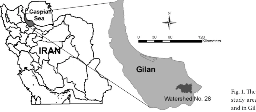
Study area. Watershed basin No. 28, part of the Hyrcanian forests of Iran, is situated in eastern Gilan Province in the south-west of the Caspian Sea (Fig. 1).

The study region covers approximately 24,000 ha. Ele-vation ranges from 0 to 2,900 m a.s.l. and slope varies from 0 to 250%. The study area is flat in the north and rugged mountains cover southern parts. This region has a temperate climate and precipitation (the mean annual precipitation is about 1,400 mm) is distributed throughout the year (Sagheb Talebi et al. 2003).

Hyrcanian forests are mixed and uneven-aged deciduous forests. Spot cutting in limited areas has been applied in these forests.

Research data.Data used in this study were: – Digital 1:25,000 thematic-topographic maps

pro-duced in 1982, which were extracted based on 1:20,000 aerial photos acquired in 1967 according to the Iranian Forests, Rangelands and Watershed Organization (FRWO) order and National Carto-graphic Centre (NCC) supervision. These maps have 63 different data layers including: residential areas, roads, railways, forests, ranges, gardens, contour lines, etc.

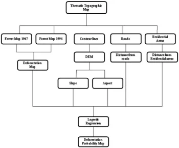
– Digital thematic-topographic maps dated 2001, which were generated based on 1:20,000 aerial photos dated 1994. These maps have 63 different data layers that are the same as in previous maps. Methodology. Deforestation mapping. The layer of forest classes was extracted from both 1967 and 1994 digital maps and then the values of 0 and 1 were labelled to non-forest and forest areas, respectively, in ArcGIS 9.3 software. This process was done for all the map sheets covering the watershed. By compar-ing forest maps related to the start and end of the period (1967 and 1994), deforestation maps were obtained. The maps were exported to Idrisi Selva software, in 30-m raster-grid format. The flow chart of the methodology and processing steps carried out in this study is shown in Fig. 2.

Explanatory variables. After extracting contour lines from the 3D digital maps of 1:25,000 scale, a digital elevation model having a spatial resolution

of 30 m was created. Slope and aspect layers were calculated using a digital elevation model (DEM). According to Beers et al. (1966) a cosine function (Eq. 1) was applied to transform the aspect into a number ranging from 0 (southwest-facing) to 2 (northeast-facing) to create a more direct measure of radiation load for statistical analysis. Distances to the nearest road and settlement were calculated as a series of buffers of 200 m expanding from each road segment and settlement centre, respectively. Road network and human settlements were derived from the digital map dated 1967. These maps were converted from vector to raster format with 30-m grid cells.

Cos (45 – Aspect) + 1 (1)

Datasets for modelling and validation. Production and validation of the logistic regression model were performed by a sampling of the geographical and environmental space of the study region. To avoid biases, the samples were balanced to have the same number of positive (deforested) and negative (non-deforested) cases (Felicisimo et al. 2002). 100 points were selected in areas presenting deforestation be-tween 1967 and 1994, and 100 points in areas that remained forested over the same period. These points should be separated by at least 1,000 m to reduce the effects of spatial autocorrelation. In this study a

sepa-Fig. 2. Flowchart of the methods and materials

Fig. 3. Forest maps of watershed basin No. 28 for 1967 (a), 1994 (b), and the deforestation map in this period (c)

ration distance of 500 m (at least 500 m) was used in-stead, because of the relatively limited area in extent (Linkie et al. 2004). Each observation is a 30-m grid cell containing either deforestation or not. 80% of ob-servations were allocated to establish the model, and 20% of them were allocated to the validation model. The model has been calibrated using a separate da-taset, to reduce the likelihood of overestimating the predictive ability of the model (Chatfield 1995; Wilson et al. 2005).

Modelling the spatial distribution of deforestation using logistic regression. To investigate the correla-tions that exist between a dichotomous dependent variable (deforested/non-deforested) and indepen-dent variables which cannot be assumed to satisfy the required assumptions of discriminant analysis (nor-mality assumption), a logistic regression model has been used (Ludeke et al. 1990). In logistic regression, a dependent variable transforms into a logit variable (the natural log of the odds of the dependent variable occurring or not), and then based on the independent variables, maximum likelihood estimation is applied to estimate the probability of occurrence of a certain event (deforestation) (Rueda 2010).

The dependent variable used for calibrating the model was derived from the analysis of two datasets of forest maps. This information was extracted from 30-m grid cells of forest layers, using Idrisi Selva soft-ware. The extraction information was exported into SPSS 16 software for further analysis. A multivariate, spatially explicit model of the deforestation was devel-oped using the logistic regression (Schneider, Pon-tius 2001; Serneels, Lambin 2001; Wilson et al. 2005). The model was used to determine the variables that explain the spatial distribution of deforestation.

A logistic model was developed based on the binary response variable (one – deforestation; zero – non-deforestation) (Rivera et al. 2012) and the explanato-ry variables (elevation, aspect, slope, distance to roads and residential areas). Before developing the model, the explanatory variables were standardized by divid-ing values by their root-mean-square because of the easier comparison of the relative effect of each vari-able (Etter et al. 2006). The logistic function gives the probability of forest loss as a function of the ex-planatory variables.

The logistic function (Eq. 2) results bounded be-tween 0 and 1 as follows:

(2)

where:

p – probability of deforestation in the cell,

E(Y) – expected value of the binary dependent variable Y,

β₀ – constant to be estimated,

β_i – predicted coefficient of each independent variable

X_i (Schneider, Pontius 2001).

The amount of the contribution of each fac-tor to deforestation is described by the regres-sion coefficients. We could transform the logistic function into a linear response with the following transformation:

p´= log_e(p/1–p) (3)

hence

p´= (β₀+ β₁ X₁+ β₂ X₂+ β₃ X₃) (4)

This transformation which allows linear regres-sion to estimate each β_i is called a logit or logistic transformation (transformation from Eq. 3 to Eq. 4). The final result is a probability score (p) for each cell (Schneider, Pontius 2001). Notice that the logit transformation of dichotomous data ensures that the dependent variable of the regression is continu-ous, and the new dependent variable (logit transfor-mation of the probability) is unbounded. Further-more, it ensures that the predicted probability will be continuous within the range from 0 to 1. The final step is the classification of these results.

Validation of the logistic regression model. To in-dicate the effectiveness and soundness of the model, statistical tests of individual predictors including goodness-of-fit statistic, and validations of predict-ed probabilities have been accomplishpredict-ed (Peng et al. 2002). At first, R square of the model was calculated. In this method, R2 _{is called pseudo R}2 _{because it is}

not computed in the same way as the regular regres-sion R2 _{(Ludeke et al. 1990). This R square indicates}

the fitness of the model, but does not give as much information as the regular regression R2 _{about the}

scatter of the data around the fitted line (Ludeke et al. 1990). The value of R2 _{is low in logistic regression}

models because of the binary response variable (Bio et al. 1998). For a very good fit of a logistic regression model, R2 _{should have values between 0.2 and 0.4}

ones (Wilson et al. 2005; Etter et al. 2006). These values range from 0.5 to 1.0. The value above 0.7 in-dicates an accurate model fit, above 0.9 inin-dicates a highly accurate model (Linkie et al. 2004) and the value of 0.5 indicates a random model.

RESULTS

The forest maps of watershed basin No. 28 for 1967 and 1994 are depicted in Fig. 3. Approximate-ly 12% (2,902 ha) of the total area was deforested during the 27-year period. Therefore, the mean an-nual deforestation rate was 0.44%.

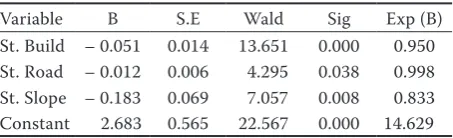
The coefficients and the value of the area under the ROC curve are listed in Table 1. During this period the probability of deforestation was significantly and negatively determined by slope (Wald = 7.057, df = 1), distance to roads (Wald = 4.295, df = 1), and distance to residential areas (Wald = 13.651, df = 1). The lo-gistic regression model proposed that deforestation is a function of slope, distance to roads and residential areas (Table 1). The coefficients for the explanatory variables indicated that the probability of deforesta-tion is negatively related to slope, distance from roads and residential areas (Table 1). Although the distance factor was found to be a contributor to deforestation, their effects are lower than those of slope.

Although the logistic regression goodness of fit measured by the Nagelkerke R2 _{statistic is low, the}

significant Chi-square value (54.12, df = 3, P < 0.001) and high correct classification percentage (72.5%) indicate the perfect fit of the model in explaining the relationship between independent and dependent variables (Table 1).

The area under the ROC curve of the model was 0.807, so this model has a good discrimination abil-ity (Linkie et al. 2004).

The best-fit model of deforestation (Table 1) was used to predict the probability of deforestation of the remaining areas of the watershed. The probability of

deforestation ranged from zero to 0.94 (Fig. 4). At the final step a classified map was generated based on the predicted probability.

DISCUSSION

The deforestation rate of the study area was 0.44% per year (2,902 ha). This study has shown the value of producing site-specific models based on logistic regression that can be used in forest management.

The deforestation models developed in this study can be used to predict future patterns of deforesta-tion and to identify where to focus stronger protec-tion for the best results. This analysis found that the spatial pattern of forest loss was dependent on several physiographic and anthropogenic fac-tors and that the logistic regression models could be used to accurately predict future deforestation trends (Linkie et al. 2004). One of these factors was slope, which was important during this period because the areas with steep slopes tended to in-clude more rugged terrain and are further from isting deforestation fronts. This may also partly ex-plain why low slope forests are the most threatened forest type (Linkie et al. 2004). We conclude that the areas with lower slopes are more accessible, and more suitable for agricultural activities that are the most important factors causing deforestation.

As expected from previous studies (Pir Ba-vaghar 2004; Wilson et al. 2005; Amini et al. 2009; Bagheri, Shataee 2010), the position of roads and residential areas were important in de-termining deforestation patterns.

Deforestation has been seen to have a negative re-lationship with slope, distance from roads and

resi-Table 1. Result of the logit analysis

Variable B S.E Wald Sig Exp (B)

St. Build – 0.051 0.014 13.651 0.000 0.950 St. Road – 0.012 0.006 4.295 0.038 0.998 St. Slope – 0.183 0.069 7.057 0.008 0.833 Constant 2.683 0.565 22.567 0.000 14.629

Chi-square value = 54.125; Nagelkerke R square = 0.383; ROC = 0.807, SE = 0.031, Sig = 0.000; Hosmer & Lemeshow test Chi-square = 7.433, Sig = 0.491; Correct classification = 72.5%, RMSE% = 23%, St. Slope, St. Build & St. Road: Standardized value of slope, distance from residential areas and roads

dential areas. Negative coefficients of these factors indicate that higher values are associated with lower probabilities of deforestation (Wilson et al. 2005; Amini et al. 2009; Bagheri, Shataee 2010). In gen-eral, a steep slope limits deforestation due to diffi-culties associated with transportation. The spatial patterns of deforestation across this area highlighted the critical role of accessibility, with the importance of distance to roads and residential areas. These re-sults reflect the findings of other deforestation as-sessments (Ludek et al. 1990; Linkie et al. 2004, 2010; Amini et al. 2009; Bagheri, Shataee 2010). It was found that 83% of deforestation occurred within a 2-km distance from roads. Similarly, Ludeke et al. (1990) also found that deforestation decreased rap-idly with a distance from roads and there was a steep drop in the percentage area deforested beyond 2 km from access routes. Wilson et al. (2005) also men-tioned that 90% of the deforested area is within 2.5 kilometres from roads.

The validation analysis showed that the explana-tory variables included in the model had a suffi-cient explanatory power to discriminate between deforested and non-deforested areas.

The correlates of deforestation may change over time and so the spatial model should be periodi-cally updated to reflect these changes. Like in any model, the quality may be improved by introducing the new variables that may contribute to explaining the spatial distribution of deforestation.

The results of this analysis are based on the as-sumption that the existing forest maps are accu-rate. Furthermore, the accuracy of this assessment relies on the quality and accuracy of the maps of the explanatory variables included in the model. These maps are the most detailed and comprehen-sive presently available for these forests.

CONCLUSIONS

This study fulfilled its aim by predicting spatial patterns of deforestation in the northern forests of Iran and understanding the underlying drivers. De-forestation is indeed as interplay between several factors. Accessibility was found to be an important variable for explaining the patterns of deforestation observed in the study area. The results indicated that slope, major roads, and residential areas have a strongly significant correlation with deforestation. So the results highlighted the critical role of acces-sibility. The results did not indicate a significant relationship with aspect and elevation. The results also showed the utility of a statistical modelling

ap-proach to analyse and predict deforestation. The logistic regression goodness of fit is low, suggest-ing that misssuggest-ing variables such as livestock’s role, might further explain differences between low and high deforestation. In spite of this, the modelling approach developed by this study would benefit conservation planning (Wilson et al. 2005; Smith et al. 2008; Linkie et al. 2010).

References

Amini M.R., Shataee Sh., Moaieri M.H., Ghazanfari H. (2009): Deforestation modeling and investigation on related physi-ographic and human factors using satellite images and GIS (Case study: Armardeh forests of Baneh). Iranian Journal of Forest and Poplar Research, 17: 431–443. (in Persian) Bagheri R., Shataee Sh. (2010): Modeling forest area decreases

using logistic regression (Case study: Chehl-Chay catchment, Golestan province). Iranian Journal of Forest, 2: 243–252. (in Persian)

Beers T.W., Press P.E., Wensel L.C. (1996): Aspect transformation in site productivity research. Journal of Forestry, 64: 691–692. Bio A.M.F., Alkemende R., Barendregt A. (1998): Determining

alternative models for vegetation response analysis: a non-parametric approach. Journal of Vegetation Science, 9: 5–16. Chatfield C. (1995): Model uncertainty, data mining and

statistical inference. Journal of the Royal Statistical Society, 158: 419–466.

Etter A., McAlpine C., Wilson K., Phinn S., Possingham H. (2006): Regional patterns of agricultural land use and defor-estation in Colombia. Agriculture, Ecosystems & Environ-ment, 114: 369–386.

Felicíslmo A.M., Francés E., Fernández J.M., González-Díez A., Varas J. (2002): Modeling the potential distribution of forests with a GIS. Photogrammetric Engineering and Remote Sens-ing, 68: 455–461.

Geist H.J., Lambin E.F. (2002): Proximate causes and underly-ing drivunderly-ing forces of tropical deforestation. Bioscience, 52: 143–150.

Laurance W.F., Albernaz A.K., Schroth G., Fearnside P.M., Bergen S., Venticinque E.M., Da Costa C. (2002): Predic-tors of deforestation in the Brazilian Amazon. Journal of Biogeography, 29: 737–748.

Linkie M., Smith R.J., Leader-Williams N. (2004): Mapping and predicting deforestation patterns in the lowlands of Sumatra. Biodiversity Conservation, 13: 1809–1818. Linkie M., Rood E., Smith R.J. (2010): Modelling the

effec-tiveness of enforcement strategies for avoiding tropical deforestation in Kerinci SeblatNational Park, Sumatra. Biodiversity Conservation, 19: 973–984.

Makinano M.M., Santillan J.R., Paringit E.C. (2010): Detec-tion and analysis of deforestaDetec-tion in cloud-contaminated Landsat images: A case of two Philippine provinces with history of forest resource utilization. In: Proceeding of the 31st _{Asian Conference on Remote Sensing (ACRS 2010):} Remote Sensing for Global Change and Sustainable De-velopment, Hanoi, Nov 1–5, 2010: 44–52.

Mertens B., Lambin E. (1999): Modelling land cover dynam-ics: integration of fine-scale land cover data with landscape attributes. International Journal of Applied Earth Observa-tion and GeoinformaObserva-tion, 1: 48–52.

Nagendra H., Southworth J., Tucker C.J. (2003): Accessibility as a determinant of landscape transformation in western Hondrus: linking pattern and process. Landscape Ecology, 18: 141–158.

Ostapowicz K. (2005): Model of forests spatial distribution in the western part of the Karpaty Mts. In: 8th _AGILE Conference on Geographic Information Science, Estoril, May 26–28, 2005: 611–617.

Peng C.J., Lee K.L., Ingersoll G.M. (2002): An introduction to Logistic regression analysis and reporting. The Journal of Educational Research, 96: 3–14.

Pir Bavaghar M., Darvishsefat A.A., Namiranian M. (2003): The study of spatial distribution of forest changes in the northern forests of Iran. In: Proceedings of the Map Asia Conference, Kuala Lumpur, Oct 14–15, 2003: 1–6. Pir Bavaghar M. (2004): Forest Area Change Detection

Re-lated To Topographic Factors and Residential Areas (Case Study: Eastern Forests of Gilan Province). [MSc. Thesis.] Karaj, University of Tehran: 110.

Rafieyan O., Darvishsefat A.A., Namiranian M. (2003): For-est area change detection using ETM+ data in northern forest of Iran. In: The First International Conference on Environmental Research and Assessment, Bucharest, Mar 23–27, 2003: 1–4.

Rivera S., Martinez de Anguita P., Ramsey R.D., Crowl T.A. (2012): Spatial modeling of tropical deforestation using socioeconomic and biophysical data. Small-scale Forestry, 12: 321–334.

Rueda X. (2010): Understanding deforestation in the south-ern Yucatan: insights from a sub-regional, multi-temporal analysis. Regional Environmental Change, 10:175–189. Sagheb Talebi Kh., Sajedi T., Yazdian F. (2003): Forests of

Iran, Research Institute of Forests and Rangelands, Forest Research Devision, Iran: 28.

Salman Mahini A., Feghhi J., Nadali A., Riazi B. (2009): Tree cover change detection through artificial neural network classification using Landsat TM and ETM+ images (case study: Golestan Province, Iran). Iranian Journal of Forest and Poplar Research, 16: 495–505.

Schneider L.C., Pontius R.G. (2001): Modelling land-use changes in the Ipswich watershed, Massachusetts, USA. Agriculture, Ecosystems & Environment, 85: 83–94. Serneels S., Lambin E.F. (2001): Proximate causes of land

use change in Narok District, Kenya: a spatial statistical model. Agriculture, Ecosystems & Environment, 85: 65–81. Smith R.J., Easton J., Nhancale B.A., Armstrong A.J., Cul-verwell J., Dlamini S., Goodman P.S., Loffler L., Matthews W.S., Monadjem A., Mulqueeny C.M., Ngwenya P., Ntumi C.P., Soto B., Leader-Williams N. (2008): Designing a trans-frontier conservation landscape for the Maputaland centre of endemism using biodiversity, economic and threat data. Biological Conservation, 141: 2127–2138.

Wilson K., Newton A., Echeverria C., Weston Ch., Burgman M. (2005): A vulnerability analysis of the temperate forests of south central Chile. Biological Conservation, 122: 9–21.

Received for publication July 8, 2014 Accepted after corrections March 26, 2015

Corresponding author:

Assistant Prof. Mahtab Pir Bavaghar, University of Kurdistan, Faculty of Natural Resources,