Finite Element Modeling of Variable Membrane Thickness
for Field Fabricated Spherical (LNG) Pressure Vessels
Oludele Adeyefa, Oluleke Oluwole
Department of Mechanical Engineering, University of Ibadan, Ibadan, Nigeria Email: [email protected]
Received January 29, 2013; revised March 2, 2013; accepted March 9,2013
Copyright © 2013 Oludele Adeyefa, Oluleke Oluwole. This is an open access article distributed under the Creative Commons Attri-bution License, which permits unrestricted use, distriAttri-bution, and reproduction in any medium, provided the original work is properly cited.
ABSTRACT
This study investigated thickness requirements for field fabricated (large) spherical liquefied natural gas (LNG) pres-sure vessels using the finite element method. In the FEM modeling, 3-dimenisonal analysis was used to determine thickness requirements at different sections of a 5-m radius spherical vessels based on the allowable stress of the mate-rial as given in ASME Section II Part D. Shallow triangular element based on shallow shell formation was employed using area coordinate system which had been proved better than the global coordinate system in an earlier work of the authors applied to shop built vessels. This element has five degrees of freedom at each corner node-five of which are the essential external degrees of freedom excluding nodal degree of freedom associated with in plane shell rotation. Set of equations resulting from Finite Element Analysis were solved with computer programme code written in FORTRAN 90 while the thickness requirements of each section of spherical pressure vessels subjected to different loading conditions were determined. The results showed membrane thickness decreasing from the base upwards for LNG vessels but con-stant thickness for compressed gas vessels. The obtained results were validated using values obtained from ASME Sec-tion VIII Part UG. The results showed no significant difference (P > 0.05) with values obtained through ASME Section VIII Part UG.
Keywords: LNG; FEM; Field Fabricated Pressure Vessels; Shell Thickness; Modeling
1. Introduction
Over the past few decades, world consumption of LNG has increased more than five-fold and it is predicted that this growth will continue to be very strong. The growing demand from large markets such as China and India combined with the increasing popularity in a large num-ber of other smaller markets has resulted in the develop-ment of many new LNG facilities throughout the world. There are significant natural gas reserves globally and exploration companies are rapidly developing facilities for exporting the natural gas with corresponding receiv-ing facilities bereceiv-ing planned and built in emergreceiv-ing mar-kets. With a timeframe of some 5 - 10 years required for planning and construction, there is currently much activ-ity underway in the LNG supply chain in preparation for current and predicted demands. Because of its unexam-pled advantages such as less floor area covering, high- pressure capability and transport facilitates, Spherical pressure vessels used for storage of gas and liquefied gas more widely than other storage tanks in the oil, gas,
chemical and other fields.
design and stress modeling in spherical vessels using global and area coordinate systems in the finite element modeling. Different design specifications and selection procedures have been outlined [7,8]. Construction of shop built spherical [9] and field fabricated cylindrical vessels have being carried out [10], however, there is still intense interest in the designing of spherical pressure vessels [11-13]. Work has proved the area coordinate system for triangular shell elements reliable and easy to use than the global coordinate system [5,6]. Thus the area coordinates system was applied in this modeling.
2. Methodology
2.1. Finite Element Modeling
Finite element analysis was used in this work. The analy-sis of this system required transformation into a discrete mathematical system [14]. The simplified structural model consisted of discrete structural elements (4 ele-ments) as opposed to the system used in an earlier method [4,5] which needed fine meshing to converge to a stress level. The approximate behavior of each element
was expressed in terms of selected generalized stress and strain variables using elasticity theory. The elements were then assembled by enforcing equilibrium of forces and compatibility of displacements at the nodes on the model. These conditions were expressed as a set of non- homogenous linear equations in which the variables were element forces and structural displacements and the con-stant terms were the applied loads [14].
2.2. Displacement Functions
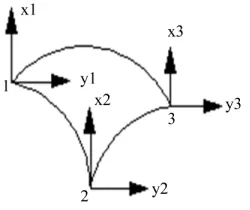
The use of shallow triangular element (Figure 1) and “area coordinates” was made use of in this work to rep-resent the transverse displacement, w, as a polynomial function of degree 3 as given by [15]. Linear polynomial equations were then used to represent the membrane dis-placements u and v using area coordinates, resulting in a constant strain triangle for the membrane action. The assumed displacement equations are:
1 1 2 2 3 3
ua L a L a L (1)
4 1 5 2 6 3
va L a L a L (2)
7 1 8 2 9 3 10 1 2 11 2 3 12 3 1
2
13 1 2 1 2 3 3 1 3 2 3 3
2
14 1 2 1 2 3 3 1 3 2 3 3
2
15 1 2 1 2 3 3 1 3 2 3 3
1
3 1 1 3 1 3
2
1
3 1 1 3 1 3
2
1
3 1 1 3 1 3
2
w a L a L a L a L L a L L a L L
a L L L L L L L L
a L L L L L L L L
a L L L L L L L L
(3)
x w
y
(4)
y w x
(5) where
2 2
2
k j i
i l l
l
and i is the length of the side opposite node i. The modified interpolation for displacement is taken as
l
Pa
(6) to determine constants as, known displacements at nodes are substituted and the equations become
1
C
a (7)
where
is the nodal degrees of freedom, C1 is inverse of transformation matrix and [a] is vector ofin-dependent constants.
2.3. Strain-Displacement Equations
Strain-displacement relationships for shallow thin shells as given by [16] are simplified for the shallow shell and expressed as follows in curvilinear coordinates.
2
2
2 2
2
, ,
, 2
x y x
y xy
u w v w w
k
x r y r x
w w
k k
x y y
(8)
The above strain Equation (8) can be written in matrix form after necessary substitutions of u, v and w in Equa-tions (1)-(3) into the above strain equaEqua-tions.
2.4. Stresses in a Curved Triangular Element
Figure 1. Shallow triangular element.
unknown function of two variables [14]. It is represented as shown below [4]:
2 6 , b m M N t t
(9)
where: M is the moment per unit length, M and
b
is the bending stress at the surface.
N is force per unit length and m which is membrane stress.
2.5. Strain Energy
The strain energy equation for an isotropic linear shell as given by [17] was adopted in this work;
2
2
2
2 2 2
2 1
1
2 1 d d
2
t
t A
x y x y xy
E U v v v
d x y (10)where, thickness of the shell, Poisson’s ratio and Modulus of elasticity
t
andv
E are the strain
and shear strain notations.
After substitution for strains in the above expression and integration with respect to , the strain energy can be separated into the membrane energy and the bending energy .
m
U
b
U
m
UU Ub (11)
2
2 2
21
2 1 d
2 2 1
m x y x y x
A
Et
U e e ve e v e
v
y x yd
(12)
3
2 2 2
2
1
2 1 d
2 24 1
b x y x y
A Et
U k k vk k v k
v
xy x yd(13) The potential energy, U W where W represents
the work done by the external load on the system. In the finite element method, the potential energy of a shell is expressed as: 1 n k k
(14)where k is the potential energy of the kth element.
2.6. Stiffness Matrix
T 1 T
d
m A m m
k t C
B D B A C 11
(15)
T 1 T
d
b A b b
k t C
B D B A C m
(16)
kmand kb are element stiffness matrices due to membrane and bending stresses respectively Dm and Db are elasticity matrices for membrane and bending stresses respectively Bm and Bbare strain matrices for membrane and bending stresses respectively.
Therefore, element total stiffness matrix is
b
kk k (17) The element stiffness matrices were then combined to give the system stiffness matrix. The stiffness matrices kb and km in terms of area coordinates were using three Gauss quadrature points. To integrate explicitly, the in-tegral equation below as it is in [6] was very useful.
1 2 3
! ! !
d 2
2 !
a b c
A
a b c L L L A
a b c
(18)where is the area of triangular element
2.7. Consistent Load Vector
It is well known fact that the best and accurate approach for dealing with distributed loads in FEM is the use of a consistent load vector which is derived by equating the work done by the distributed load through the displace-ment of the eledisplace-ment to the work done by the nodal gen-eralized loads through the nodal displacements. The shal-low triangular shell element acted upon by a distributed load q per unit area in the direction of w, has work done by this load given by:
1 d d
A
P
qw x y (19)where w is:
1
w P a P C (20) and
P for the present element is given as
0 0 0 0 0 0 1 2 3 1 2 2 3 3 1 13 14 15
P
L L L L L L L L L P P P
where
2
13 1 2 1 2 3 3 1 3 2 3 3
2
14 1 2 1 2 3 3 1 3 2 3 3
2
15 1 2 1 2 3 3 1 3 2 3 3
1
3 1 1 3 1 3
2 1
3 1 1 3 1 3
2 1
3 1 1 3 1 3
2
P LL L L L L L L
P L L L L L L L L
P L L L L L L L L
and is as defined in Section 2.2.
t nodal generalized The work done by the consisten
force through the nodal displacements
is given by:
T
2
P F (22) Hence, from Equations (19)-(22),
ob
the nodal forces were tained
T
1 T d d
F C
P q x y (23) Equation (23) gives the nodal forces on aan
e ready for solution, they
sp
toring LNG
wing simulation pa
e 70
Specified Minimum Yield stress = 260 MPa
single element; d the nodal forces for the whole structure were obtained by assembling the elements’ nodal forces.
2.8. Boundary Conditions
Before the system equations ar
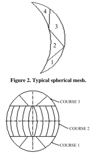
must be modified to account for the boundary conditions of the problem. For this system, it was assumed that dis-placements in all directions with the exception of radial direction are zero. Also, due to the symmetry nature of the system, 1/6 of the spherical vessel (Figure 2) was used thereby reducing computing time. Shown (Figure 2) is sample of meshing of 1/6 of the spherical vessel with 4 elements and 6 nodes as used in this work.
Figure 3 shows the arrangement for the elements in the herical shell. Course 1 takes thickness of Element 1. The lower and upper portions of Course 2 take thicknesses of Elements 2 and 3 respectively while Course 3 has thickness corresponding to the thickness of Element 4.
2.9. Cases Considered
Case 1: Storage Tank S
For a spherical vessel with the follo
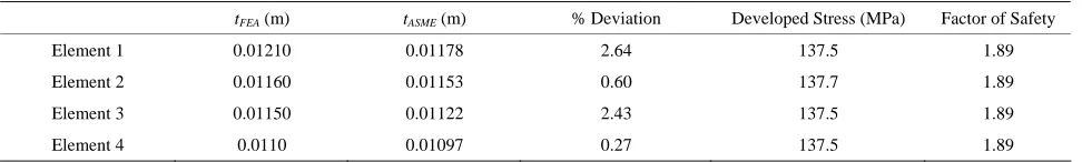
rameters, the thickness of each element corresponding to the membrane stress developed at the centroid was determined (Table 1). Membrane stresses at the centroid were deliberately programmed to be within the range of 0.5% and 0.8% less than the spherical vessel construction material allowable stress given by ASME standard to avoid a rise over the allowable membrane stress.
[image:4.595.342.495.83.341.2]Design Internal Pressure = 600 KN/m2 Density of Stored Product = 560 Kg/m3 Material of Construction = A516M Grad Material Allowable Stress = 138 MN/m2
Figure 2. Typical spherical mesh.
Figure 3. 3-course version spherical vessel. Material Factor of safety = 1.88
Radiu
Case 2: as
sponding to the
mem-br etermined for
sp em-
br
3.
T veloped stress
oring LNG and values were explicitly s of Spherical Vessel = 5.0 metres
Storage Tank Storing Compressed G
Thickness of each element corre
ane stress developed at the centroid was d
herical vessels storing compressed gas (Table 2). M ane stresses at the centroid were deliberately program- med to be within the range of 0.5% and 0.8% less than the spherical vessel construction material allowable stress to avoid a rise over the allowable membrane stress.
Internal Design Pressure = 600 KN/m2 Material of Construction = A516M Grade 70 Material Allowable Stress = 138 MN/m2
Pa Specified Minimum Yield stress = 260 M Material Factor of safety = 1.884 Radius of Spherical Vessel = 5.0 metres
Results and Discussions
ables 1 and 2 show the thicknesses and de values obtained for storage vessels st compressed gas respectively. These
Table 1. Element thicknesses for spheric vessel storing liquefied product (LNG).
t t ) Factor of Safety
al
FEA (m) ASME (m) % Deviation Developed Stress (MPa
Element 1 0.01210 0.01178 2.64 137.5 1.89
Element 2 0.01160 0.01153 0.60 137.7 1.89
Element 3 0.01150 0.01122 2.43 137.5 1.89
Element 4 0.0110 0.01097 0.27 137.5 1.89
T Element thi pherical v toring compresse
[image:5.595.55.539.203.385.2]t Factor of Safety
able 2. cknesses for s essel s d gas.
FEA (m) tASME (m) % Deviation Developed Stress (MPa)
Element 1 0.01090 0.01087 0.275 137.5 1.891
Elem nt 2 e 0.01090 0.01087 0.275 136.3 1.908
Element 3 0.01090 0.01087 0.275 137.0 1.898
[image:5.595.57.286.435.515.2]Element 4 0.01090 0.01087 0.275 137.0 1.898
[image:5.595.61.282.560.660.2]Figure 4. Element thicknesses for spherical vessel storing liquefied product (LNG).
Figure 5. Developed stresses in spherical vessel storing liq-uefied product (LNG).
Figure 6. Element thicknesses for spherical vessel storing compressed gas.
ould also be seen from Tables 1 and 2 that the thick- nesses calculated for each element are in close agreem specified minimum yield stress given by ASME code. It c
ent
Figure 7. Developed stresses in spherical vessel storing compressed gas.
with ASME values. The maximum percentage deviation from the thicknesses using FE model and ASME is
deliberately programming the allowable stress to be
ally Coupled BEM-FEM and Comparison with Test Results,” Earthquake Engineering and Structural Dynamics, Vo 9-124.
doi:10.1002/(SICI)1096-9845(199802)27:2<109::AID-E 2.64%. This percentage value is reasonable as the results showed no significant difference (P > 0.05). The wisdom in
within the range of 0.5% and 0.8% less than the spherical vessel construction material allowable stress could be seen here because all the stress values fall a little below the allowable membrane stress. The FE model in this research work also proved that it is possible to obtain reasonable results with few elements using area coordi-nates as opposed to the large number of elements needed for the model developed by Adeyefa et al. [5] using global coordinates. Thus the use of area coordinates allow an easy modelling of variable vessel thickness which would otherwise would have become impossible using global coordinates.
REFERENCES
[1] H. M. Koh, J. K. Kim and J. H. Park, “Fluid-Structure Interaction Analysis of 3-D Rectangular Tanks by a Variation
l. 27, No. 2, 1998, pp. 10
[2] Y.-S. Choun and C.-B. Yun, “Sloshing Analysis of Rec- tangular Tanks with a Submerged Structure by Using Small-Amplitude Water Wave Theory,” Earthquake En- gineering and Structural Dynamics, Vol. 28, No
pp. 763-783.
. 7, 1999,
6-9845(199907)28:7<763::AID-E doi:10.1002/(SICI)109
QE841>3.0.CO;2-W
[3] J. Dong, et al., “Numerical Calculation and Analysis of Single –Curvature Polyhedron Hydro-Bulging Process for Manufacturing Spherical Vessels,” Institute of Nuclear Energy Techno
[4] O. A. Adeyefa and O. O. Oluwole, “Finite Element Mod eling of Stress Distribu
logy, Tsinghua University, Beijing, 2005.
tion in Spherical Liquefied Natur
_2.pdf
.
e and I.-S. Yoon,
ld Gas Con-
_vessel
essel Junction Dissertation, Texas
0.
-al Gas (LNG) Pressure Vessels,” Proceedings of the Nige-rian Institute of Industrial Engineers, Nigerian Institute of Industrial Engineers, Abuja, 2011, pp. 65-78.
[5] O. A. Adeyefa and O. O. Oluwole, “Finite Element Ana- by t lysis of Von-Mises Stress Distribution in a Spherical
Shell of Liquified Natural Gas (LNG) Pressure Vessels,”
Engineering, Vol. 3, No. 10, 2011, pp. 1012-1017. [6] O. A. Adeyefa and O. O. Oluwole, “Finite Element Mod-
eling of Shop Built Spherical (LNG) Pressure Vessels,”
Engineering, Unpublished, 2013.
[7] AIJ, “Design Recommendation for Storage Tanks,” 2011. www.aij.or.jp/jpn/databox/2011
[8] Kolmetz, “Storage Tanks Selection and Sizing,” 2011.
http://kolmetz.com/pdf/EDG/ENGINEERING_DESIGN_ GUIDELINE__storage_tank_rev
[9] Wilco, “Spherical Compressed Natural Gas Vessels,” 2012 www.wilcofab.com/wilcocompressedn.html
[10] Y.-M. Yang, J.-H. Kim, H.-S. Seo, K. Le
“Development of the World’s Largest Above-Ground Full Containment LNG Storage Tank,” 23rd Wor
ference, Amsterdam, 5-9 June 2006, pp. 1-14. [11] EGPET, “LPG Spherical Storage Tank Design,” 2012.
www.egpet.net/vb/threads/25114Sphericalstoragetank [12] Wikipedia, “Storage Tank,” 2012.
http://en.wikipedia.org/wiki/Storage_tank [13] Wikipedia, “Pressure Vessel,” 2012.
http://en.wikipedia.org/wiki/Pressure [14] S. I. Mahadeva, “Analysis of a Pressure V
he Finite Element Method,” Ph.D. Tech University, Lubbock, 1972.
[15] O. C. Zienkiewicz and R. L. Taylor, “The Finite Element Method Set,” 5th Edition, Vol. 2: Solid Mechanics, But- terworth-Heinemann, Oxford, 200
[16] E. Reissner, “On Some Problems in Shell Theory,” Pro-ceedings of 1st Symposium on Naval Structural Mechan-ics, California, 11-14 August 1958.