Online Full Text



Abstract— Mammography is a special type of low-powered x-ray method that has been used to improve diagnostic and decrease the number of unneeded biopsies. Detection breast cancer in early stage can help treatment successful. Many researches show that malignant breast tumors tend to demonstrate irregular and undulated shapes, whereas benign breast tumors are regularly round and smooth shapes. Consequently, many researches about tumor shape may help in maintaining diagnosis. Thus, the contour feature of tumor contour is very significant feature to distinguish between malignant and benign tumor. In this paper, we propose an approach to automatically appraise the density and contrast of breast images using gamma correction to increase the intensity of dense pixels with light intensity and vice versa to decrease the sparse intensity pixels showing dark intensity. In the segmentation process, we use region growing technique to get region of interest. We also extract three important features including texture, shape, and intensity histogram. In the classification process, we use SVM to classify tumor into two classes: malignant and benign. Moreover, we also compare between three features by combines and separate these features for SVM classification. The results of classification shows that when we combine the shape feature in the classification process, it can be able to correctly classify two types of mammography images and we obtained the high accuracy more than using only texture features and intensity features.

Index Terms—feature selection, image classification,

mammography, support vector machine.

I. INTRODUCTION

Breast cancer is a dangerous type of tumor originated from breast tissue, and it accounts for 23% of all cancers in women. The most effective way to detect breast cancer is through the breast mammogram screening, ultrasound images [1]-[7], and also magnetic resonance [5]-[7]. Mammography is the most common imaging technique to detect breast cancer. However, the major limitation for mammography diagnosis is sensitivity due to interpreting mammography is a labor-intensive task for radiologists who cannot always offer stable results during interpreting [8].

K. Chaiyakhan is with the Computer Engineering Department, Rajamangala University of Technology Isan, Muang, Nakhon Ratchasima, Thailand (corresponding author to provide phone: +66868129127; e-mail: [email protected]).

N. Kerdprasop is with the School of Computer Engineering, Suranaree University of Technology, Muang, Nakhon Ratchasima, Thailand (e-mail: [email protected]).

K. Kerdprasop is with the School of Computer Engineering, Suranaree Universiyof Technology, Muang, Nakhon Ratchasima, Thailand (e-mail: [email protected]).

The interpreting depends on experience, training, and subjective criteria. Actually, about ten percent of all malignant tumors in mammography are missed by radiologists, and ninety percent of the missed tumors are dense area of breast tissue. It is also admitted that expert radiologists can miss a significant proportion of abnormal tumors. On the contrary, a large number of diagnosed abnormal tumors turn out to be benign after biopsy. Many methodologies have thus been proposed to solve this uncertain interpretation problem by providing assistance to the advanced cancer detection and diagnosis tools

During the last year, several algorithms have been proposed for breast density segmentation. The statistical approach has been proposed by [9]. They provide connected density clusters taking the spatial information of the breast tissue into account. Quantitative and qualitative results show that their approach is able to correctly detect dense breasts apart from other tissue types. A methodology that based on modeling a set of patched of either fatty or dense parenchyma using statistical analysis has been presented by [10]. They analyze two different strategies to perform this modeling process such as principal component analysis and linear-discriminant based model. Once the tissue models have been learned, each pixel of a new mammogram is classified based on neighborhood information as being fatty or dense tissue.

Malignant breast tumors are characterized by cluster of cells indicating uncontrolled outgrowth that leads to penetrate surrounding tissue [11]. The penetration of malignant tumors tends to spread an irregular tumor contour, which will be displayed in mammography as irregular, undulated and ill-defined contour, whereas benign tumors have a uniform outgrowth, round and smooth contour. Hence, it is significant that the contour feature will affect better result of classification.

In our proposed method, we use gamma correction to enhance the image contrast. In segmentation process we use a well-known region growing method to find the ROI and then crop the image to consider only the tumor region. This process will speed up the subsequent classification process because unnecessary background has been removed. After that we extract three types of feature such as texture [12], intensity histogram and shape feature [13]. After that we input digital data to the classification process. The performance of the proposed image classification approach has been evaluated by comparing the accuracy between three features that we extracted after preprocessing image.

Feature Selection Techniques for

Breast Cancer Image Classification with

Support Vector Machine

II. MATERIALS AND METHODS A. Gamma Correction

Gamma correction is the name of nonlinear operation used to code and decode luminance (or brightness level) on an image. It can also enhance contrast of the image. The luminance value is between 0 and 1, where 0 means absolute darkness (black), and 1 is the brightest (white). Different camera devices do not correctly capture luminance and do not display luminance precisely. Therefore, we need to correct them using gamma correction function. Images which are not corrected can look either light region darker or dark region lighter. Suppose a computer monitor has 2.2 power function as intensity to voltage response. This just means that if we send a message to the monitor that a certain pixel should have intensity equal to x, it will actually display a pixel with intensity equal to . Because the range of voltages sent to monitor is between 0 and 1, it means that the intensity value displayed will be less than what we want it to be. Fig. 1 illustrates the gamma correction model which has been computed from a formula given in (1).

₍₁₎

where  is the encoding or decoding value. If value of  < 1, it is called and encoding gamma or gamma compression, conversely if  > 1, it is called a decoding gamma or gamma expansion. The effect of gamma correction on an image if  >1 is that shadow in that image will be darker because the mapping weighs toward lower (darker) output values. If  < 1, dark region will be lighter because the mapping biases toward higher (brighter) output values. Fig. 2 illustrates this relationship. The two transformation curves show how values are mapped when gamma that is less than and greater than 1. In each graph, the x-axis demonstrates the intensity values of the input image, and the y-axis is the intensity values in the output image.

Gamma correction

1/2.2

CRT gamma 2.2

0.5

0.218

0.5

0.218

Fig. 1. Gamma correction model.

top

bottom

low high

top

bottom

low high

<1 >1

Fig. 2. Two different gamma correction settings.

B. Region Growing

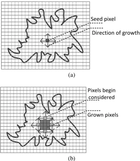
Region growing is a simple region-based image segmentation method using pixel information to adjust the seed point initialization. Small areas in an initial set are iteratively merged according to similarity constraints. The seed point selection starts by choosing an arbitrary pixel and compare it with neighboring pixels that have similar value. After that, increase the size of the region. When the growth of one region stops, then simply choose another seed pixel that does not yet belong to any region and start the process again. The process stops when all pixels belong to some region. Fig. 3 shows the example of region growing.

Direction of growth Seed pixel

(a)

Pixels begin considered

Grown pixels

(b)

Fig. 3. The example of region growing.

Region growing determines the region of object directly. The basic formulation is shown in (2). This equation states that the segmentation completes when every pixel is in a region and the points in the regions must be disjoint. Equation (3) states the property that the pixels must be in a segmented region. Equation (4) constrains that regions and are different in the sense of predicate .

⋃

(4)

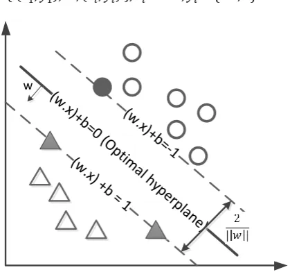
C. Support Vector Machine

that maximizes the distance between the two parallel hyperplanes. An assumption is made that the larger of this margin, the better of data classification.

We consider 2 datasets of the form in (5).

{ } { } (5)

(w

.x) +

b =

₁

(w

.x)+

b=-

₁

(w

.x)+

b=0

_(O

ptim

al h

ype

rpla

ne)

w

Fig. 4. Optimal hyperplane with maximum margin.

where l denotes the total data instances, i denotes the sequence of data, m is number of dimensions, and y is a class label (+1 or -1) to denote each group of data after separation process. If the training data are linearly separable, we classify each data instance as either positive, or negative based on the computation given in (6). In this equation, w denotes weight of data vector on the separation line, x1 is

positive data vector, and x2 is negative data vector.

where, yi = +1

III. PROPOSED WORK

In the proposed work, we have divided our process into five main parts: image preprocessing, segmentation, feature extraction and classification. Fig. 5 shows the framework of this research.

A. Image Preprocessing

Mammogram images usually have noises due to disturbances like Gaussian noise or some little darkness and brightness noise called salt and pepper noise. In this paper, we use median filter to remove these noises. Median filter is a nonlinear method effectively used for removing noise while retaining edges. It works by moving the little window called filter that moves pixel by pixel through the image and changes the pixel value to be the median of neighboring pixels. The median is calculated by first sorting all the pixel values from the filter into numerical order, and then picking the middle pixel value. The output of this de-noising step is the clearer image without noise.

The next step of image preprocessing is image enhancement. We adjust the brightness and darkness of

images using gamma correction algorithm. Fig. 6 shows the original images of malignant and benign cases comparing to the improved results after applying the gamma correction technique. The gamma correction helps contrasting the tumor area from the fatty area. In Fig. 6(b), we can see that the tumor area has lighter intensity and density than the original image. In Fig. 6(d), after gamma correction process, the area of benign tumor is lighter than original image. If we compare between Fig. 6(b) and Fig. 6(d), they are rather different because Fig. 6(b) is the malignant case and it has more light and dense intensity pixels than those in Fig. 6(d) which is a benign case.

Segmentation Pre-Processing

Mammogram Images

Image Enhancement (Gamma Correction)

ROI (Region Growing) De-noising (Median Filter)

Feature Extraction

Texture Feature

Shape Feature

Intensity Histogram Feature

Classification

Support Vector Machine

Evaluation

Malignant Benign

Fig. 5. The framework of the proposed system.

(a) (b) (c) (d)

B. Segmentation

The segmentation process separates the tumor areas from the background tissue in mammogram images. In this step, we apply the region growing segmentation method. Region growing is a region-based method starting with seed points in the image, and then propagating seeds until the specified stopping criteria are satisfied. Appropriate seed point selection is important. Therefore, in our proposed work, we select seed point using the centroid of object computed from area and position of object (centroid), as shown in (7) and (8).

∑ ∑

(7)

̅ ∑ ∑

̅

∑ ∑

(8)

where W is the white pixel in the image and i, j are the position of white pixel. After the region growing process, we will get the region of interest (ROI, white pixels) and then we crop only the ROI (Fig. 7) to removing background that may affect the classification and clustering process.

(a) (b) (c)

Fig. 7. The result of region growing and the cropped image: (a) gamma corrected image, (b) the image after applying region growing technique, (c) cropped image.

C. Feature Extraction

The objective of feature extraction step is to represents the image in its reduced and compact form in order to facilitate and speed up the decision making process such as classification and clustering. In this paper, we extract three types of features: texture, shape, and intensity histogram features.

1) Texture Features

Texture is one of the important features used in identifying objects in an image. Texture features are based on gray-level co-occurrence matrix (GLCM), also known as the gray-level spatial dependence matrix. The GLCM function characterizes the texture of an image by calculating how often pairs of pixels with specific values and in a specified spatial relationship occur in an image. We create a GLCM, and then extract statistical measures from this matrix such as contrast, correlation, and homogeneity in four directions (0o, 45o, 90o, 135o). We use these properties of texture to input into the classification process.

2) Intensity Histogram Features

The shape of the intensity histogram features provides several information to describe the properties of the image. Six statistic features obtained from the histogram are mean, variance, skewness, kurtosis, energy, and entropy. The mean is the average intensity level, whereas the variance is the variation of intensities around the mean. The skewness shows whether the histogram is symmetric. The histogram is symmetrical if the skewness is zero. For asymmetric cases, it is skewed above the mean if the skewness is positive, and skewed below the mean if the skewness is negative. The kurotosis is a measure of whether the data are peaked or flat relative to a normal distribution. Data with high kurtosis tend to have a distinct near the mean, and having heavy tails. Data with low kurtosis tend to have a flat top near the mean. Entropy is a metric to measure magnitude of disorder in a system.

3) Shape Features

In this process, we extract shape feature using the percentage of curvature. First we drag lines from centroid to every edge pixel and measure distance and angle from centroid to every edge pixel. After that, we plot the graph with angle along the x-axis and distance on the y-axis. From the graph, we can notice difference of curvature due to the distinct shape of malignant and benign tumor. We also do the normalization to find the percentage of curvature. As a result, we get the different percentage of curvature between malignant and benign tumor. We observe that malignant tumor shows many serrate along its contour and we can get the higher percentage of peak in this graph. In contrast, in the case of benign tumor, it has fewer serrate than the malignant contour. Fig. 8 illustrates example of curvature measurement. Fig. 9 shows the different graph of curvature between malignant and benign contour.

q q

(a) (b)

Fig. 8. Measuring the curvature: (a) malignant contour (b) benign contour.

D. Classification

………..100100110010101001000110111000111011000111……….. (a)

………..100000000000100000000000100000100000000100……….. (b)

Fig. 9. Graph of curvature: (a) malignant contour (b) benign contour.

IV. EXPERIMENTAL RESULTS

In this proposed work, we use data set from DDSM (Digital Database for Screening Mammography). We have selected from DDSM 190 images that include both cases of tumor, that is, malignant and benign (malignant case consists of 110 images and benign case consists of 90 images). This work has been implemented using MATLAB. We run our experiments on a core i5/2.4 GHZ computer with 4 GB RAM.

TABLEI

Classification results between features.

Features Accuracy (%) AUC

Texture, Shape, Histogram (TSH) 89.47 0.89 Histogram, Shape (HS) 87.37 0.87

Texture, Shape (TS) 85.26 0.84

Histogram, Texture (HT) 81.58 0.79

In the classification process, we compare between features using SVM classifier. The results are illustrated in Table I.

It can be noticed from the classification results summarized in Table I that the classification accuracy recognizing the benign and malignant images of the SVM (with RBF – radial basis kernel function) using combination between three features (texture, shape and intensity histrogram) represents the highest rate at 89.47%. In other three combining features as shown in Table I, the

accuracy are 87.37%, 85.26% and 81.58%, respectively. We can conclude from this result that our proposed work using three types of feature and SVM classification has a higher accuracy than using only texture feature and intensity histogram feature.

We also show in Fig. 10, the area under curve (AUC) of the four features combination: TSH, HS, TS and HT have the AUC value, 089, 0.87, 0.84 and 0.79, respectively. The higher the AUC value indicates the more precise detection of true positive cases with less inclusion of unwanted false positive.

Fig. 10. Area under curve of four combination features.

V. CONCLUSIONS

Mammography classification using support vector machine with image enhancement and three types of extracted features that we proposed in our framework is the main contribution of this paper. Image enhancement using gamma correction can improve contrast of mammogram images to be seen clearly. After the image enhancement process, we extract the region of interest (ROI) using a well-known algorithm called region growing that can help the cropping of only the tumor object and at the same time eliminating the unnecessary background. After the ROI extraction, the three types of image features including texture, shape, and intensity histogram can be constructed. The processed images are then sent as input to the classification process using SVM with RBF kernel. The classification accuracy of SVM using all three features, especially when add the shape feature (89.47%) is higher than the other (87.37%, 85.26% and 81.58%).

REFERENCES

[1] S. Huber, J. Danes, I. Zuna, J. Teubner, M. Medl, and S. Delmore, “Relevance of sonographic B-mode criteria and computer-aided ultrasonic tissue characterization in differential diagnosis of solid breast masses,” Ultrasound in Medicine and Biology, vol. 26, no. 8, pp. 1243-1252, Aug. 2000.

[2] G. Rahbar, A.C. Sie, G.C. Hansen, J.S. Prince, M.L. Melany, H.E. Reynolds, V.P. Jackson, J.W. Sayre, and L.W. Bassett, “Benign

versus malignant solid breast

masses: US differentiation,” Radiology, vol. 213, no. 12, pp.889-894, Dec. 1999.

[3] P. Skaane, “Ultrasonography as adjunct to mammography in the evaluation of breast tumors,” Acta Radiologica Supplementum , vol. 40, no. 420, pp. 1-47, Dec. 1999

[4] M.A. Dennis, S.H. Parker, A.J. Klaus, A.T. Stavros, T.I. Kaske, and S.B. Clark, “Breast biopsy avoidance: the value of normal mammograms and normal sonograms in the setting of a palpable lump,” Radiology, vol. 219, no. 1, pp.168-191, 2001.

[5] W.A. Berg, L. Gutierrez, M.S. NessAiver, W.B. Carter, M. Bhargavan, R.S. Lewis, and O.B. Ioffe, “Diagnostic accuracy of mammography, clinical examination, US, and MR imaging in preoperative assessment of breast cancer,” Radiolo-gy , vol. 233, no. 3, pp. 830-849, 2004.

[6] M.J. Collins, J. Hoffmeister, and S.W. Worrell, “Computer-aided detection and diagnosis of breast cancer,” Seminars in Ultrasound, CT and MRI, vol. 27, no. 4, pp.351-355, 2006.

[7] M.L. Giger, “Computerized analysis of images in the detection and diagnosis of breast cancer,” Seminars in Ultrasound, CT and MRI, vol. 25, no. 5, pp.411-418, 2004

[8] F. Maes, D. Vandermeulen, and P. Suetens, “Medical image registration using mutual information,” Proceedings of the IEEE, vol. 91, no. 10, pp. 1699-1722, 2003.

[9] A. Oliver, X. Llado, E. Perez, J. Pont, E. Denton, J. Freixener and J. Marti, “A statistical approach for breast density segmentation,”

Journal of Digital Imaging, vol.23, no.5, pp.527-537, 2010.

[10] D. Brzakovic, N. Vujovic, M. Neskovic, P. Brzakovic and K. Fogarty, “An approach to automated detection of tumors in mammograms,”

IEEE Transaction in Medical Image, vol.9, no.3, pp.233-241, 1990. [11] Y.H. Chou, C.M. Tiu, G.S. Hung, S.C. Wu, T.Y. Chang, and H.K.

Chiang, “Stepwise logistic regression analysis of tumor features for breast ultrasound diagnosis,” Ultrasound in Medicine and Biology, vol. 27, no. 11, pp.1493-1498, Nov. 2001.

[12] A.V. Alvarenga, W.C.A. Pereira, A.F.C. Infantosi, and C.M. Azevedo, “Complexity curve and grey level co-occurrence matrix in the texture evaluation of breast tumor on ultrasound images,” Medical Physics, vol. 34, no. 2, pp. 379-387, 2007

[13] W.C. Pereira, A.V. Alvarenga, A.F. Infantosi, L. Macrini, and C. E. Pedreira, “A non-linear morphometric feature selection approach for breast tumor contour from ultrasonic images,” Computer in Biology and Medicine, vol. 40, 2010.

Kedkarn Chaiyakhan is currently

a Ph.D. student in the School of Computer Engineering, Suranaree University of Technology, Thailand. She received her bachelor degree in Computer Engineering from Rajamangala University of Technology Thanyaburi in 1998 , master degree in Computer Engineering from King Mongkut’s University of Technology Thonbuti in 2007. Her current research includes image classification and image clustering.

Nittaya Kertprasop is and

associate professor at the School of Computer Engineering, Suranaree University of Technology, Thailand. She received her bachelor degree in Radiation Techniques from Mahidol University, Thailand, in 1985, master degree in Computer Science from the Prince of Songkla University, Thailand, in 1991 and doctoral degree in Computer Science from Nova Southeastern University, U.S.A, in 1999. She is a member of ACM and IEEE Computer Society. Her research of interest includes Knowledge Discovery in Databases, Artificial Intelligence, Logic Programming, and Intelligent Databases.

Kittisak Kerdprasop is an