Light Induced Gravity Phonons

(1)

https://www.scirp.org/journal/jmp ISSN Online: 2153-120X ISSN Print: 2153-1196

DOI: 10.4236/jmp.2019.1014110 Dec. 17, 2019 1674 Journal of Modern Physics

Light Induced Gravity Phonons

Philipp Kornreich1,2

1_{1090 Wien, Austria} 2_{King of Prussia, PA, USA}

Abstract

Einstein theorized that a mass travels towards another mass, not because it is attracted by a force acting across a distance, but because it travels through space and time that is warped by masses and energy. Einstein postulated that this space-time fabric can have wave-like modes which have been measured by the LIGO experiment. A consistent model of the generation of space-time-fabric-modes by a light Photon is derived for slight space-time deformations. Each Photon generates a shower of very small amplitude space-time fabric modes. Each mode can have a number of energy quanta. The probability of a Photon generating a shower of space-time modes is much larger than the probability of all the space-time modes collecting and generating a Photon. Therefore, this process has a unique Arrow of Time. Similar to the energy quanta of displacement modes in an elastic medium which is called Phonons, the energy quanta of the space-time fabric modes are called gravity Phonons. Both are tensor waves. Gravity Phonons have spin angular mo-mentum of 2 and propagate with the speed of light. At every step of these calculations, equations derived from the General Relativity Theory by scien-tists and verified by Astronomical observations or experiments are employed.

Keywords

Photons, Phonons, Gravity, General Relativity, Space-Time, Generation Rate, Arrow of Time

Note

In the whole paper numbers such {8} in curly brackets denote equation num-bers in the literature.

1. Introduction

Einstein [1]theorized in 1916 that a test mass travels towards a mass not because it is attracted by a force that acts across a distance between masses, but because How to cite this paper: Kornreich, P.

(2019) Light Induced Gravity Phonons.

Journal of Modern Physics, 10, 1674-1695. https://doi.org/10.4236/jmp.2019.1014110

Received: August 9, 2019 Accepted: December 14, 2019 Published: December 17, 2019

(2)

DOI: 10.4236/jmp.2019.1014110 1675 Journal of Modern Physics

the test mass travels through space and time that is warped by mass and energy. In this paper, the Interaction of a light Photon with a space-time fabric that has been deformed by a non-rotating Earth-like mass is described. The de-rivation is only for a slightly curved space-time fabric.

A light Photon will not interact to first order with flat space-time, the ordinary four-dimensional Minkowski space. The Earth-like mass is used to remove this symmetry and facilitate the interaction of the Photon with warped space-time.

Einstein also postulated the existence of wave modes in the space-time fabric. This has been verified by the Laser Interferometer Gravity-Wave Observatory LIGO experiment [2]. The interaction of a Photon with warped space-time fa-bric generates space-time modes, which can have any number of energy quanta, called gravity Phonons. The energy quanta of displacement modes in an elastic medium are called Phonons. Because of the similarity of the interaction of light and Phonons, to the interaction of light and the space-time modes, the space-time mode energy quanta are called gravity Phonons. The gravity Pho-nons valid for slight deformation of the space-time fabric only, are different from Gravitons which presumably are valid for all values of gravity. In this paper, the gravity Phonons have an energy of 0.59893 atto eV and a wavelength of 1.7298 A. U. These small values are expected since the derivation is based on astronomical observations and experiments.

In this paper, equations derived from the General Relativity Theory (GRT) and verified by astronomical observations or experiments are employed at every step of the calculations.

Professor Paul Sutter of Ohio State University and Chief Scientist of the COSI Science Center [3] asks “Why Can’t Quantum Mechanics Explain Gravity?” Quantized models exist for the other three forces, the Electromagnetic Force, the Weak Nuclear Force, and the Strong Nuclear Force. In this paper, a quantized formulation of Einstein’s [1] space-time fabric modes is presented for slightly curved space-time fabric. Thus, now there exists quantized models for all four forces, a Gravity Force for slightly curved space-time fabric only, the Electro-magnetic Force, the Weak Nuclear Force and the Strong Nuclear Force of the standard model of Physics.

This discussion involves space-time which permeates all space at all times, a light electromagnetic wave, and a large non-rotating mass. The mass used has the same value as the mass of the Earth. The derivation is in four steps:

FIRST, to model the affect of the slightly warped space-time on an electro-magnetic wave, Einstein’s description [1] of the deflection of a light wave by the curvature of space-time due to a mass is used. This has been verified by observ-ing the deflection of a light beam passobserv-ing close to the Sun by F. W. Dyson et al. [4].

(3)

by the GRT. The GRT has been proven correct in all its tests. Therefore, the affect of the energy of the light wave on the curvature of space-time, predicted by the GRT, must also be correct.

THIRD, a Taylor series expansion to second order of the time dilation equa-tion is used for the derivaequa-tion of the frequency ω of the light wave in the pres-ence of gravity as a function of the frequency ωE of the light wave in the

ab-sence of gravity and the space-time mode frequency ωG. The gravitational blue

shift of the frequency, in this case, of gamma rays emitted by iron 57

Fe samples mounted a vertical elevation of 22.5 m apart has been measured by R. V. Pond and J. L. Sinder [7].

In the FOURTH step, Quantum Electrodynamics [8] is used to formulate a Hamiltonian from the above described frequency relationship in second quan-tized form.

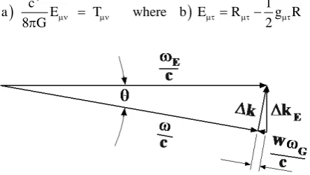
A momentum vector diagram illustrating the affect of the curvature of space-time on a light wave, and the affect of the energy of the light wave on the curvature of the space-time fabric to within a constant for slightly curved space-time fabric only, as shown in Figure 2 is derived. The values of the change of the light wave momentum and momentum of the light wave generated space-time fabric modes are functions of the deflection angle of the light wave.

This derivation is not valid in the vicinity of large masses such as Black Holes and Neutron Stars. It is also not applicable to the Early Universe, where the mass density was much larger than it is now, and the affect of gravity was larger.

The space-time fabric, described by the second rank metric tensor has a simi-larity to an elastic fabric, described by the fourth rank elastic constant tensor. The metric tensor that describes the curvature of the space-time fabric is itself a function of the coordinate components of space-time. The elastic constant ten-sor is constant. The elastic fabric mode energy quanta are called Phonons. The electromagnetic field mode and space-time mode interactions are similar to the quantized electromagnetic field and acoustic mode interaction [9]. Because of this similarity the energy quanta of the space-time fabric modes are called “gravity Phonons”.

The gravity Phonons are massless Bosons, that propagate with the speed of light. Light Photons are derived from a vector model, the Maxwell Electromag-netic Theory, and have a spin angular momentum of 1. The gravity Phonons are derived from a tensor model, the GRT, and have a spin angular momentum of 2. The space-time deformation caused by the mass acts as a cavity to determine the frequency of the space-time fabric modes.

Before Ludwig Boltzmann [10] in 1896, continuous wave theories were used to formulate Statistical Thermodynamic models of acoustic and electromagnetic modes. But none of these formulations agreed with observations. First Boltzmann

(4)

the vicinity of Black holes or Neutron stars, the space-time fabric is only slightly deformed.

Therefore, the gravity Phonons derived here can be used for the calculations of statistical Thermodynamic properties of the space-time fabric such as its av-erage energy, entropy, pressure, and temperature (2.72503˚K). The thermal energy of 0.2340247 meV of the Cosmic Background Radiation is much larger than the energy of a gravity Phonon of 0.59893 atto eV calculated here. The cal-culations of the Statistical Thermodynamic models are deferred to future publi-cations.

A. D. Sakharov [12] of the Sovietski Academii Nauk (Soviet Academy of Science) and later H. E. Puthoff [13] postulated that gravity is not a basic force. It is a consequence of the electromagnetic force, where the electromagnetic force is generated by a Zero Point Fluctuation of the vacuum. The electromagnetic force can also be generated by a Zitterbewegung, Jitter Motion in German, of particles. However, we are not concerned with the basic phenomena that generate electro-magnetic waves. But, like Sakharov and Puthoff, we are concerned with the con-tribution to the deformation of the space-time fabric by the energy of an elec-tromagnetic wave.

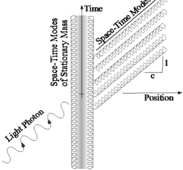
Each light Photon generates a shower of identical space-time modes, see

Figure 1. Each space-time mode can have any number of energy quanta, called gravity Phonons. Quantum Mechanics is a probabilistic model of Nature. The probability of generating a space-time mode shower is much larger than the probability of all the gravity Phonons collecting and generating a Photon. The entropy of the shower of gravity Phonons is much larger than the entropy of the electromagnetic wave that created the gravity Phonon shower. Therefore, this process has a unique Arrow of Time.

This Arrow of time is consistent with Arthur Stanley Eddington’s [14] concept of the Arrow of Time. Another explanation for the discussion of the Arrow of Time, are in References [15][16] and [17]. Stephen Hawking [18] discusses the Arrow of Time in “The Beginning of Time” based on the way the Universe de-veloped. This is very different from the Arrow of Time of the gravity Phonons. The gravity Phonons model developed here is also not valid for the beginning of the Universe discussed by Hawking.

The reciprocal relationship between electromagnetic wave modes and gravity is similar to the reciprocal interaction between sound waves and gravity dis-cussed by Nicolis and Penco [19] in “Mutual Interaction of Photons, Rotons, and Gravity” and A. Esposito [20] et al. in “Gravitational Mass Carried by Sound Waves”. Instead of a reduction of the symmetry of the space-time fabric, they use a non-linear sound wave effect. The model described in this paper does not have to resort to Plank time or Plank length, or other exotic parameters.

(5)

[image:5.595.281.465.77.248.2]

DOI: 10.4236/jmp.2019.1014110 1678 Journal of Modern Physics Figure 1. The annihilation of a light Photon generates a shower of

iden-tical space-time modes. Each space-time mode can have any number of energy quanta called gravity Phonons. A stationary Mass causes a distor-tion of the space-time fabric, which facilitates the interacdistor-tion of the pho-ton and the space-time modes. The distortion of space-time by the mass can also be expressed in terms of standing space-time waves. Also, both the light Photon and gravity Phonons propagate with the velocity of light. This derivation is for slightly curved space-time fabric only fields only.

introduction of a local inertial frame. In this paper, we also use a second-order expansion approach in our derivations.

Bryce C. DeWitt attempts to derive a Quantum theory of gravity from the GRT starting with a General Relativistic Lagrangian. His derivation is intended to be applicable for all gravity values. He wrote 3 papers [22] [23] [24] but he was unable to produce a Quantum Mechanical model of gravity in a form that has useful applications.

The model derived in my paper corresponds approximately to DeWitt’s limit Hamiltonian H∞ appearing in equation {4.9} on page 1119 of Quantum Theory of Gravity I. DeWitt is using the full tensor formulation of the GRT for his derivation. I use contractions with time-like unit vectors of the tensors in the GRT which results in a scalar formulation of the GRT. The contraction leaves only functions that were verified by astronomical observations or experiments because most of the tests that validated the GRT were based on calculations that reduced parameters of the GRT to scalars. This results in a description that is similar to an Empirical description of physical observations. Since my derivation is from equations validated by real physical observations and experiments it su-persedes any difficulties that occur in the full quantization of the GRT.

Carlo Rovelli [25] in his paper “Notes for a Brief History of Quantum Gravity” describes in detail the history of formulizing Quantum gravity in the time period from 1930 to 2001. Rovelli describes three main approaches to the formulation of Quantum Gravity.

(6)

Nieu-DOI: 10.4236/jmp.2019.1014110 1679 Journal of Modern Physics

wenhuizen, and others, found firm evidence of a non-renormalizability model, a search for an extension of the GRT using a renormalizable perturbation expan-sion was started. A high order derivative theory and supergravity theory con-verged successfully to string theory.

The SECOND was an attempt to construct a quantum theory in which the Hilbert space carries a representation of the operators corresponding to the full metric, or some functions of the metric, without a background metric to be fixed. The formal equations of the quantum theory were successfully formulated with loop quantum gravity.

The THIRD was an attempt to use some version of Feynman’s functional integral quantization to define the theory. This is somewhat similar to the ap-proach used in this paper.

The paper “Potential Origin of a Quantitive Equivalence between Gravity and Light” by Michael A. Persinger [26] is even more speculative. It invokes a mass of the Photon and the mass of the universe to calculate the pressure of Photons in the Universe.

The research described above and in references [21] through [27] are attempts to formulate a quantized gravity mode model that is generally applicable. The Quantized space-time fabric modes derived in this manuscript, are based only on an interaction of an electromagnetic wave and a weak gravitational field. It does not require renormalization and is not based on String Theory or Loop Quantum Gravity [25] [28]. The model of space-time fabric quantization de-scribed in Chapter V of this paper is used for the calculation of the gravity Pho-non generation rate by Solar radiation.

2. Reciprocal Interaction of Space-Time Modes and a Light

Wave

NOTE: This derivation is only valid for slightly curved space-time fabric. The effect of the curvature of the space-time fabric on a light wave is to deflect it as Einstein [1] described. To describe the affect of the energy of the light wave on the curvature of space-time, Einstein’s equation is used. In Einstein’s equa-tion, the Einstein tensor describes the curvature of space-time, and the affect of the light wave energy is described by the electromagnetic stress tensor.

The deflection of a light wave by the curvature of space-time due to the Solar mass is calculated in Einstein’s Chapter “On the Influence of Gravitation on the Propagation of Light” in section §4 “Bending of Light-Rays in the

Gravitation-al Field” on page 108 and page 168, equation {74}. The deflection angle [1] θ__is:

)

ss

)

ss

2

2M G r r

a b c

R R

c R

θ =  θ =   ≡

 



Schwarzschild ratio (1)

Here M_ is the solar mass, R_ =6.957 1 m× 08 is the radius of the Sun and

ss 2954.03

r_ = 0552 m is its Schwarzschild [29] radius. G is Newton’s

gravita-tional constant.

ss 2

2M G r

c

= 

(7)

For the Sun the Schwarzschild ratio ss 6

4.24612 0

r

R 7 1

−

= ×

 

and the deflection

angle θ =_ 0.8758266 arc seconds. It was first measured by F. W. Dyson, A. S. Eddington, and C. Davidson [4] in 1919. Subsequent measurements have con-firmed the value of the deflection angle. For the Earth rss = 8.869518 mm is the

Schwarzschild radius and R = 6.378 × 106_{m is the radius. For the Earth, the} Schwarzschild ratio rss _1.390642 9

R 10

−

= × . The deflection angle of a light beam θ = 0.286841 marc seconds which corresponds to slightly curved space-time.

The wave vector E c ω

of the light wave in the absence of gravity, the wave

vector c

ω_{of the light wave subject to gravity, and change in the wave vector}

∆k of the light wave due to the deflection by gravity form the large triangle in

Figure 2. Similar to equation 1b, this deflection angle θ is approximately equal to the Schwarzschild ratio rss

R .

)

ss

)

ss E

E E E

r r

c k c k c k

a sin b c d k

R cR

ω

∆ ∆ ∆

θ = θ ≈ ≈ ∆ ≈

ω ω ω (3)

Dadhigh Naresh [6] writes in “Subtle is the Gravity” Section 5, that since energy and mass are equivalent in the GRT, the energy of the light wave also contributes to the curvature of the space-time fabric. The affect of the light elec-tromagnetic wave on the curvature of space-time can be calculated from Eins-tein’s equation [5]. To date, all astronomical observations and experimental measurements have verified the accuracy of the GRT. The affect of the energy of the light wave on the curvature of space-time is very small. I could not find any astronomical observation or experimental measurements of this affect. However, since the affect is predicted by the GRT which has been proven correct in all its tests, the affect of the energy of the light wave on the curvature of space-time must also be valid.

)

c4

)

1

a E T where b E R g R

[image:7.595.263.485.526.651.2]

8 Gπ µν = µν µτ = µτ−2 µτ (4)

(8)

Eµν is the Einstein tensor derived from the Ricci tensor Rµν. Tµτ is the electromagnetic part of the stress-energy tensor. Here gµτ is the metric tensor. The Ricci tensor is derived by a contraction over the indices ρ_and σ_{of the}

Riemann-Christoffel tensor Bρ_µστ. The curvature of space-time is described by the Riemann-Christoffel tensor. Equation (4) is a tensor equation. It can be re-duced to a scalar equation for slightly curved space-time fabric only by con-tracting Equation (4) with a time like unit vector with components uµ.

)

4

tt tt

4

c 1

a R u u g u u R T u u

8 G 2

c

b R T

8 G c

c Curvature Electromagnetic energy density function

8 G

µ τ µ τ µ τ

µτ µτ µτ

 ₋ ₌

 

π  

− ≈

π

= π

(5)

Summation over repeated Greek indices is implied. No summation over the Latin indices t is implied. Ett and Ttt are the tt components of the Einstein

tensor and Stress Energy tensor. Here the Ttt component of the Stress Energy

tensor is equal to the electromagnetic energy density function. The timelike unit vector uµ is:

[

]

uµ = −1 0 0 0 (6)

The development of Einstein’s equation resulting in Equation (5b) is de-scribed in detail by Lee Loveridge in “Physical and Geometric Interpretations of the Riemann Tensor, Ricci Tensor and Scalar Curvature”, Reference 5. Loveridge gives an excellent description of the derivation of the Einstein equation from the concept of curvature of space-time, the Riemann-Christoffel Tensor, and the Ricci Tensor. Loveridge uses the sum over the coordinates of a large number of point particles in the vicinity of the original point particle under consideration. Summing over a large number of particles is equivalent to the contraction of the Riemann-Christoffel tensor to form the Ricci tensor. Instead of describing the motion of a single point particle one has now to describe the motion of a volume

V

δ _{of all the point particles in the vicinity of the original point particle. From} Loveridge’s [5] equation {7} one can express the left side of Equation (5b), in the form of second time derivatives of the volume δV in a three-dimensional space.

( )

2

4 2

Mass only

2 2 2 2

0 0

D V

c 1 D V 1

Q t

4 G V c dt V c dt

 δ δ 

−  − =

π   (7)

where Q t

( )

is the electromagnetic energy density function. Loveridge also de-rives Newton’s laws from the Einstein equation, Equation (4). The electromag-netic energy density function Q t

( )

in the real world is a function of space and time. A constant and uniform electromagnetic energy density would result in a constant, uniform and therefore, isotropic space-time fabric deformation. But the electromagnetic field does not interact with an isotropic space-time fabric.

( )

(9)

( ) ( ) ( )

2

4 2

Mass only

2 2 2 2

o 0 o

D V k c

c 1 D V 1

d q exp j t

4 G V c dt V c dt V

∞

−∞

 δ δ  ∆ ψ

−  − = ψ ψ ψ

π  

∫



(8)

where j= −1. Here q

( )

ψ is a dimensionless Fourier Integral of the elec-tromagnetic energy density function and ψ_{is a frequency. A detailed} deriva-tion of the electromagnetic stress tensor and its contracderiva-tion is derived in Ap-pendix A. Equation (A4b) is used in the argument of the Fourier integral on the right sides of Equations (8). Expressing the incremental volume δV also as Fourier integrals.

)

( )

)

Mass only o

( )

a For curved space-time V d V t exp j t

b For curved space-time due to mass only V d V exp j t

∞ −∞

δ = ψ ψ

∫

(9)

where V t

( )

is a very slow varying function of time. By substituting Equations (9) into Equation (8).

( )

_{( )}

( ) ( ) ( )

2 2 2

2 2

o

V t

c D D

exp j t d exp j t d

4 G dt V dt

k c

d q exp j t

V ∞ ∞ −∞ −∞ ∞ −∞  

− _ ψ ψ − ψ ψ_

π  

∆ ψ

= ψ ψ ψ

∫



(10)

Performing first, the differentiation of the terms in the square bracket of Equ-ation (10). The volume amplitude V t

( )

in the first Fourier Integral in the square bracket of Equation (10) is a very slow varying function of time com-pared to the oscillation. Therefore, it is treated as a constant in the Fourier Integral. Taking the inverse Fourier Integral:

( ) ( )

2 2 G 2 G G G G

o o o o

k c

V V

c V

2 j q

4 G V V V V

∆ ω

₋ ₋ ω ₊ω _{− ω} ₌ _ω

 

π  



 

(11)

where ωG is an oscillating frequency of a Fourier component of the incremental

volume δV. Therefore, ωG is also an oscillating frequency of the space-time

fa-bric modes. Since the volume V t

( )

is a very slow varying function of time, the first term in the square bracket of Equation (11) has been neglected. The Vo-lume V in the third term in the square bracket of Equation (11) was approx-imated by Vo. Collecting the remaining terms of Equation (11).

( ) ( )

2 G G G o o k c c V j q

2 G V V

∆ ω ω

− = ω

π

 _

(12)

Assuming the volume V has also a harmonic time dependence. Therefore, one can approximate the first time derivative V of V in Equation (12) by:

2 ss

2 G q R

V j w

r c

π

≡ 

 ₍₁₃₎

where 3

s

43

s

1.060763 10 2 G R

m second

c r

− π

= ×

 _{and where the dimensionless}

(10)

G

ss

R

k w

r c

ω

∆ = ₍₁₄₎

The disturbance of the space-time fabric with wave vector G c ω

propagates in

the opposed direction to the deflected wave, see Figure 2. The smaller triangle of

Figure 2 is illustrated by Equation (14), describes the affect of the energy of the light wave on the curvature of space-time to within a constant w. The large tri-angle of Figure 2 describes the affect of the curvature of space-time on the light wave. By substituting Equation (14) into Equation (3d) one obtains for the ratio of the oscillating frequency ωG of the space-time fabric mode and the

fre-quency ωE of the light in the absence of gravity.

)

G ss E

)

G ss2

2

ss E

r r

wR

a b

c r cR wR

ω ω ω

≈ ≈

ω (15)

For the Earth ss2 2

18 1.938138404 r

R 10

−

= × _{is as expected, a very small number.}

Equations (3) and (14) describe the reciprocal relationship of the light wave and the space-time fabric. Equation (15b) describes the combined affect of the space-time curvature acting on the light wave and the energy of the light wave acting on the space-time curvature.

3. The Relationship between the Frequency of the Light

Wave Subject to Gravity, the Frequency of the Light Wave

Not Subject to Gravity and the Frequency of the

Space-Time Modes

The electromagnetic energy density is employed for deriving a Hamiltonian of the electromagnetic mode and space-time fabric modes in second quantized form. The electromagnetic energy density has a quadratic form in the compo-nents Fµν of the electromagnetic field tensor. Therefore, in order to derive the Hamiltonian, a quadratic form of a function of the small Schwarzschild ratio

ss r

R is obtained from a Taylor series expansion of the gravitational time dilation [1] equation.

The other General Relativistic affect used, is that clocks run slower when clos-er to the centclos-er of gravity of a mass than at largclos-er distances from the mass [1][7]. Clocks use oscillators, such as pendulums or vibrating crystals as the timing elements. Thus, the frequency of an oscillator is lower when closer to the center of gravity of a mass. The oscillating frequency of the light wave behaves like the oscillating frequency of the clock oscillators. This affect has been experimentally verified by measuring the gravitational blue shift of the frequency of gamma rays emitted by iron 57

Fe by R. V. Pond and J. L. Sinder [7].

(11)

Bending of Light Rays. Motion of the Perihelion of a Planetary Orbit.” on page 160 using g44 from equation {70}. This equation for g44 is also the

Schwarz-schild metric [30] or Schwarzschild solution. The frequency ω of a light wave in a gravitational field as a function of the frequency ωE of the light wave in the

absence of the gravitational field φ_{can be derived from the time dilation}_[1]_.

a) E

2

2 1

c

ω ω =

φ −

form ref. [31] b) MG R

φ = − resulting in c) E ss

r 1

R

ω ω ≈

+

(16)

Equation (16c) can also be calculated from the dilation of the oscillating pe-riod of a harmonic oscillator derived in “Relativistic Harmonic Oscillator” by Kirk T. McDonald [32] of the Joseph Henry Laboratory, of Princeton University. He calculated the time deletion of the period of oscillation of a mass and a spring oscillator in a gravitational field. When one reverses the approximation used to derive Professor McDonald’s equations {8} and {12} in his paper [32] one ob-tains Equation (16c). Another reference for the gravitational time dilation from which one can derive the function of the frequency ω_{in a gravitational field,}

as a function of the frequency ωE of the light wave far from the mass in the

absence of the gravitational field is given in “Gravitational Time Dilation” in Wikipedia [33]. Expanding Equation (16c) to second order in a Taylor series in the small parameter rss

R to obtain a quadratic equation.

2 ss ss

E 2

r 3r

1

2R 8R

 

ω ≈ ω _ − + + _

  (17)

This is the quadratic form of the function of the small Schwarzschild ratio ss

r

R discussed above.

The smaller the distance R, the closer the light wave is to the center of gravity of a mass, and the stronger is the affect of gravity acting on the light wave. The smaller the distance R, the lower the oscillating frequency ω_{of the light wave.}

The light frequency is “Red Shifted”. Recall that in stronger gravity, clocks run slower, and the light wave oscillates slower.

Here rss

R represents the distortion of the curvature of the space-time fabric by the mass which facilitates the interaction of the light wave and the space-time fabric.

Substituting Equation (15b) into Equation (17) one obtains for the frequency ω of the light wave near the surface of an Earth like mass:

)

E G G

E

2

G G

E

wω ω 3wω

a ω ω

2 8

wω 5wω

b ω ω

4 16

≈ − + +

 

≈_ − _ +

 



(18)

Putting the last term 5w G 16

ω

(12)

the remaining equation by -Plank’s constant divided by 2π, and taking the square root.

G E

w 4

ω ω ≈ ω − 

  (19)

The constant w in Equations (18) and (19) will have to be evaluated from ob-servations.

4. Formulation of the Second Quantized Form of the

Space-Time Modes

Next, a second quantized Hamiltonian is derived from the square root of the energy _ω_{of the light wave in the presence of gravity of Equation (19), as a}

function of:

the square root of the energy ωE of the light wave in the absence of gravity,

the energy w G 16

ω

 _{of the space-time fabric modes,}

and the energy term 5w G 16

ω

 _{that was set aside in Equation (18).}

The Quantum Electrodynamics models described in “Quantum Electronics” by Amnon Yariv [34] in the section on “Plane Wave Quantization” equations {5.6.15} on page 98 are employed for the electric field vector operator E

( )

ω

and the magnetic flux density pseudo vector operator B

( )

ω as functions of the

light frequency in the presence of gravity. These operators are also described in reference [35]equations {2.12}, {2.13}, and {2.52}; and also in reference [36].

) ( )

( )

(

)

) ( )

( )

(

)

jkz jkz

E

o

jkz jkz

o B

ˆ

a j S e e

2V

ˆ

and b S e e

2V

− −

ω

ω = −

ε ωµ

ω = +

a a



E a r

B a r

†

(20)

where εo is the dielectric constant of free space, µo is the permeability of free

space, aˆx is a unit vector. S

( )

r is a normalized description of the space-time

distribution of the electromagnetic field modes and V is the volume occupied by the light Photons. By substituting Equation (19) for ω into Equations (20).

) ( )

( )

(

)

( )

(

)

) ( )

( )

(

)

( )

(

)

G

jkz jkz jqz jqz

E E E G

o

G

jkz jkz jqz jqz

o

B E E G

w ˆ

a j S e e S e e

2V 4

w ˆ

b S e e S e e

2V 4

− −

 ω 

ω =  ω − − − 

ε _ _

 ω 

µ

ω =  ω + − + 

 

 

a a b b



E a r r

B a r r

† †

(21) where the form factors SE and SG are normalized.

)

_Volume E E

)

_Volume G G

1 1

a 1 S S dv b 1 S S dv

V V

∗ ∗

=

_∫

=

_∫

(22)

The form factors SE and SG are calculated by using post-Newtonian

(13)

Photon mode operators

a

and †

a are associated with the square root

E

ω

 of the energy ωG, and gravity Phonon mode operators b and †

b

are associated with the square root w G

4

ω

 _{of the energy}w _G

16 ω

 _{. The}

space-time energy quanta, gravity Phonons form a Hilbert space. The Photons also form a Hilbert space. The state raising and state lowering operators on these Hilbert spaces are defined as:

†

a is the light Photon number state raising operator;

a

_{is the light Photon number state lowering operator;}

†

b is the gravity Phonon number state raising operator;

b is the gravity Phonon number state lowering operator.

The state raising and state lowering operators, which operate on the light Photon and gravity.

Phonon number state wave functions n and m , are given below. Where

n=0,1, 2, 3, 4,, m=0,1, 2, 3, 4,

)

† †

nk m

a n n 1 n 1 e m m 1 m 1

b n n n 1 f m m m 1

c 0 0 g 0 0

d n k h m

= + + = + +

= − = −

= =

= δ = δ

a b

 

(23)

The light Photon operators

a

_and †

a commute with the gravity Phonon operators. b and †

b The commutation relation for the light Photon opera-tors

a

_and †

a as well as the commutation relation for the gravity Phonon operators b and †

b are:

)

† †

)

† †

a aa −a a=1 b bb −b b=1 (24)

The electromagnetic energy density u is described by John David Jackson [37]

in “Classical Electrodynamics”, Chapter 6, section 6.7 equation {6.106} on page 259, and by L. D. Landau and E. M. Lifshitz [38] in “The Classical Theory of Fields” equations {31.1} and {31.5} on page 76. The total electromagnetic energy U is:

)

0 0 Volume

o o

o Volume

o

1 2 1

a U F F F F dv

2 2

B B 1

b U E E dv

2

β αµ

β µα

α α α α

 

= _ − _

µ µ

 

 

= _ ε + _

µ

 

∫

(25)

where MKS units were used. The electromagnetic field tensor with components Fαβ is described by Jackson [37]in equation {11.137} on page 556, and by Lan-dau and Lifshitz [38] equation {23.5} on page 61, and also in equations {5} and {6} of Reference [39]. Substituting equations 21 into equation 25b, similar to the derivation of the Hamiltonian of equation {5.6-10} by Yariv [34], to obtain the total Hamiltonian H operator. The derivation of the Hamiltonian operator H is performed in Appendix B.

Substituting Equations (24) into Equation (B3) of Appendix B for †

(14)

†

bb , adding the term 5w G 16

ω

 _{of Equation (18b), back in, and performing the}

integration using Equations (22).

( ) ( )

† E

j k q z j k q z

E G † †

G E E G

Int.Vol. Int. † G 1 2 w

S S S S

1

dv e e

V 2 2

w 3 8 ∗ ∗ − − −  

= ω _ + _

 

ω ω

+ _ _

− _ + _

ω  

+ _ + _

∫

a a

b a ba

b b    H (26)

Equation (26) represents the three terms of Equations (17) and (18a). Equa-tion (26) contains three sub Hamiltonian operators, an Electromagnetic wave Hamiltonian operator HE, an Interaction Hamiltonian operator HInt, and a

gravity wave Hamiltonian operator HG:

)

(

)

( )

₍

₎

( )

)

†

E E

j k q z j k q z

† †

G E E G

Int _Int.Vol G G G

Int. † G G 1 a 2

S S S S

1

b dv N e N e

V 2

w

c 3 8

∗ ∗

− − −

 

= ω _ + _

 

+

− _ _

= ω _ + _

ω  

= _ + _

∫

H H H    a a

b a b a

b b

(27) Equation (27b) implies that each Photon interacts with NG fold degenerate

space-time fabric modes. Each of these space-time fabric modes can have any number m of energy quanta, gravity Phonons. The number NG is derived from

the term w G E

2

ω ω

in Equations (18a) divided by ωG and Equation (15b).

)

G E E

)

E

)

G

G G G ss ss

w 1 1 R wR

a b c N

2w 2 w 2 w 2r 2r

ω ω ω ω

= = ≈

ω ω ω (28)

For an Earth-like mass NG = 1.79773024 × 108. The quantity S SG E S SE G

∗₊ ∗

is always real. The two operators in the Interaction Hamiltonian operator HInt

of Equation (27b) describe the reciprocal actions of the electromagnetic and gravity waves. The terms in the Interaction Hamiltonian operator HInt define;

either that a light Photon is annihilated and NG identical gravity Phonon

modes are created in a forward traveling wave j k q z( )

e− − , or NG gravity

Pho-nons spontaneously assemble and are annihilated, and a light Photon is created in a reverse traveling wave j k q z( )

e − . Therefore, each light Photon generates a shower of NG identical space-time modes, see Figure 1. Each space-time

mode can have any number of energy quanta, gravity Phonons.

The Interaction of the electromagnetic wave and gravity wave are restricted to the volume where both are present. This is the Interaction volume VInt.

Quantum mechanics is a probabilistic model of Nature. The probability that a light Photon is annihilated and NG gravity Phonons are created, is much

(15)

assem-DOI: 10.4236/jmp.2019.1014110 1688 Journal of Modern Physics

ble and create a light photon. This process exhibits a unique Arrow of Time

[15][17]. From Equation (27c) the gravity Phonon ground state is:

G G

3w

0 0

8 = _ω

H (29)

The total energy and momentum before and after the interaction must also be conserved.

E G G G

3w N

8

ω = ω − ω + ω

    (30)

where ω_{of Equation (18) is the frequency in the presence of gravity.}

Substi-tuting Equation (15b) for ωG into Equation (30). 2 ss ss

E 2

r 3r

1

2R 8R

 

ω = ω _ − + _

 

  (31)

Equation (31) is in agreement with Equation (17).

5. Calculation of the Gravity Phonon Generation Rate

Fermi’s Golden Rule is employed to calculate the average rate

_{( )}

E

1

τ ω at which

the light from the Sun generates gravity Phonon modes with frequency ωG.

Fermi’s Golden Rule was derived by Enrico Fermi [40] using time dependent perturbation theory in “Nuclear Physics”, and described in “Quantum Mechan-ics” by Eugene Merzbacher [41] Chapter 19 equation {19.99}.

( )

2

E Sun Int Sun

E

1 2

1 N 1 N 0

π

= ρ ω −

τ ω  H (32)

Here 1 NSun−1HInt NSun 0 is an interaction matrix element, where Sun

N is the Photon number state wave function for NSun Solar radiation

generated light Photons, and 0 is the initial gravity Phonon number state wave function. Here ρ ω

( )

E is the density of states per unit Photon energy

E

ω

 per unit volume.

) ( )

₍

_{) (}

)

) ( )

2E

E E E 2 3

E E

1 dn 1

a f b

V d 2 c

exp 1

kT

ω

ρ ω = ω ρ ω =

ω

ω π  _{ −}

 

 

 _

  (33)

The Bose-Einstein distribution function [11] is included with the density of states. The Interaction Hamiltonian of Equation (27b) includes the integral over the interaction volume. Substituting Equation (27b) and Equation (33b) into Equation (32) to obtain the gravity Phonon generation rate _{τ ω}

_{( )}

1 . The term in Equation (27b) that annihilates NG gravity Phonons and generates a light

Photon is neglected. The gravity Phonon Generation Rate is:

( )

2 2 2 Int E G G Sun

E 3 E

Sun

V N N

1

c exp 1

kT

ω ω =

τ ω _π   ω ₋ 

   

 

 

(16)

The following data is used:

E

ω = 3.755898 × 1015_{radians per second, the frequency at the peak of the} black body radiation curve for a solar temperature TSun of 5778˚K.

G

ω = 0.0072634797 radians per second calculated from Equation (15b), cor-responding to a gravity wave wavelength of 2.593318 × 1011_{m or 1.733526 A.U.}

G

N = 3.591514389 × 108 calculated from Equations (28c).

The top of the Earth atmosphere receives a Solar radiation energy density of 1361 W/m2_{. This results in a Photon density}

Sun

N = 1.144981 × 1013 Photons/m3. Setting the value of the constant w equal to 1. By substituting the numerical values into equation 34 one obtains:

( )

E 2 3 1

8

9.143898 1

m se

10 − c−

= × ⋅

τ ω and

( )

29 3

E 1.093626 10 sec m

−

τ ω = × ⋅ . By

comparison, the Plank time 44

p 5

G

t 5.391159 10 sec

c

−

=  ≈ × _.

6. Conclusions

Einstein [1] theorized in 1916 that a test mass travels towards a mass not because it is attracted by a force that acts across a distance, but because the test mass tra-vels through space and time that is warped by mass and energy. A light Photon will not interact to first order with flat space-time, the ordinary four-dimensional Minkowski space. The Earth-like mass is used to remove this symmetry and facili-tate the interaction of the Photon with warped space-time. In this paper, the Interaction of a light Photon with a space-time fabric that has been de-formed by this non-rotating Earth-like mass is described. The derivation is only for a slightly curved space-time fabric.

Einstein also postulated the existence of wave modes in the space-time fabric. This has been verified by the LIGO experiment [2]. The interaction of a Photon with the space-time fabric generates space-time modes. Each space-time mode can have any number of energy quanta, called gravity Phonons. Gravity Pho-nons are tensor waves, they are Bosons, they have a spin angular momentum of 2, and propagate with the speed of light. In this example, the space-time quanta have an energy of 0.59893 atto eV and a wavelength of 1.7298 A.U.

Slightly curved space-time fabric implies that the escape velocity of a test mass from the surface of a mass under consideration is much less than the velocity of light. It also implies that the space-time fabric mode caused by the mass can ex-pand with the velocity of light to a size that is much larger than the mass.

(17)

massless Bosons. Since the gravity Phonons are tensor waves, they have spin angular momentum 2. The shape of the deformation of space-time and the Pho-ton frequency ωE determine the space-time fabric mode frequency ωG.

As of this date, 29 October 2019, there now exists quantized models for all four forces, a Gravity Force for slightly deformed space-time fabric, the Electro-magnetic Force, the Weak Nuclear Force and the Strong Nuclear Force of the standard model of Physics. The gravity Phonons can, among other applications, be used to calculate the Statistical Thermodynamic quantities of the space-time fabric such as its average energy, entropy, pressure, and temperature (2.72503˚K), etc. The space-time mode quanta have only an energy of 0.59893 atto eV and the thermal energy of the Cosmic Background Radiation (CBR) in the Universe at a temperature of 2.72503˚K has a thermal energy of 0.23482478 meV. Therefore, the ratio of the space-time mode quanta energy of equation 29 to the thermal energy of the CBR is only 2.55054 × 10−15_{. Thus, the Ideal Gas} Law should hold for the Universe modeled as a gas, with the galaxies as mole-cules.

It should be possible to verify this model by observations since its derivation is based on astronomical observations and experiments.

Each gravity Phonon has an energy of only 0.6 atto eV. The annihilation of a light Photon generates a shower of 36,000,000 identical space-time modes. Each space-time mode can have any number of energy quanta gravity Phonons. This interaction has two forms. The Photon can generate 36,000,000 space-time modes, or the 36,000,000 space-time modes can assemble and create a Photon. Quantum Mechanics is a probabilistic model of Nature. The probability of a Photon generating a large number of gravity Phonons is much larger than the probability of a large number of gravity space-time modes assembling and form a Photon. Therefore, this process exhibits a Unique Arrow of Time. That is, the Unique Arrow of Time is a consequence of a large number of gravity Phonons necessary to create a light Photon because gravity is such a weak force.

A quantized model of space-time modes and their properties for slightly curved space-time fabric only has been derived in this paper.

Acknowledgements

I thank my wife Marlene Danzig Kornreich for her suggestions to the text, and for making the text more understandable to a reader. I also thank her for editing and working together on this manuscript.

Conflicts of Interest

The author declares no conflicts of interest regarding the publication of this paper.

References

(18)

Relativity. Dover Publishing Co., ‎Mineola.

[2] Abbott, B.P., et al. (2016) Observation of Gravitational Waves from a Binary Black Hole Merger. Physical Review Letters, 116, Article ID: 06112.

https://doi.org/10.1103/PhysRevLett.116.061102

[3] Sutter, P. (2016) Why Can’t Quantum Mechanics Explain Gravity.

[4] Dyson, F.W., Eddington, A.S. and Davidson, C. (1920) A Determination of the Def-lection of Light by the Sun’s Gravitational Field, from Observations Made at the Total Eclipse of May 29, 1919. Philosophical Transactions of the Royal Society of London. Series A, Containing Papers of a Mathematical or Physical Character, 220, 291-333. https://doi.org/10.1098/rsta.1920.0009

[5] Loveridge, L.C. (2004) Physical and Geometric Interpretations of the Riemann Tensor, Ricci Tensor and Scalar Curvature.

[6] Dadhigh, N. (2001) Subtle Is the Gravity. 21th Conference of India Association for General Relativity, Nagpur, 30 January 2001.

[7] Pond, R.V. and Sinder, J.L. (1964) Affect of Gravity on Nuclear Resonance. Physical Review Letters, 13, 539-540. https://doi.org/10.1103/PhysRevLett.13.539

[8] https://www.physik.hu-berlin.de/de/nano/lehre/copy_of_quantenoptik09/Chapter2 [9] Li, E.B., et al. (2014) Photonic Aharonov-Bohm Affect in Photon-Phonon

Interac-tions. Nature Communications, 5, Article No. 3225.

https://doi.org/10.1038/ncomms4225

[10] Boltzmann, L. (1896) Vorlesungen über Gastheorie, Vol. I. J.A. Barth, Leipzig. Boltzmann, L. (1898) Vorlesungen über Gastheorie, Vol. II. J.A. Barth, Leipzig. [11] Bose (1924) Plancks Gesetz und Lichtquantenhypothese. Zeitschrift für Physik, 26,

178-181. (In German) https://doi.org/10.1007/BF01327326

[12] Sakharov, A.D. (1968) Docladi Academii Nauk. Soviet Physics—Doklady, 12, 1040. [13] Puthoff, H.E. (1989) Gravity as a Zero-Point-Fluctuation Force. Physical Review A,

39, 2333-2342. https://doi.org/10.1103/PhysRevA.39.2333

[14] Eddington, A.S. (1928) The Nature of the Physical World. The Gifford Lecture 1927, MacMillan Company, New York.

[15] Coveney, P. and Highfield, R. (1991) The Arrow of Time.

[16] Hawking, S. (2008) A Brief History of Time. Bantam Books, New York, London. [17] Kornreich, P. (2008) Mathematical Models of Information and Stochastic Systems.

CRC Press Taylor and Francis Group, Boca Raton, 289. [18] Hawking, S. (1996) The Beginning of Time.

http://www.hawking.org.uk/the-beginning-of-time.html

[19] Nicolis, A. and Penco, R. (2018) Mutual Interaction of Photons, Rotons, and Gravi-ty. Physical Review B, 97, Article ID: 134516.

https://doi.org/10.1103/PhysRevB.97.134516

[20] Esposito, A.K. and Rafael Nicolis, A. (2019) Gravitational Mass Carried by Sound Waves. Physical Review Letters, 122, Article ID: 084501.

[21] Marsh, G.E. (2011) Electromagnetic and Gravity Waves: The Third Dimension. Argon National Laboratory, Chicago.

[22] DeWitt, B.C. (1967) Quantum Theory of Gravity. I. The Canonical Theory. Physical Review, 160, 1113-1147. https://doi.org/10.1103/PhysRev.160.1113

(19)

Theory. Physical Review, 162, 1195-1239. https://doi.org/10.1103/PhysRev.162.1195

[24] DeWitt, B.C. (1967) Quantum Theory of Gravity. III. Applications of the Covariant Theory. Physical Review, 162, 1239-1256. https://doi.org/10.1103/PhysRev.162.1239

[25] Rovelli, C. (2001) Notes for a Brief History of Quantum Gravity.

https://doi.org/10.1142/9789812777386_0059

[26] Persinger, M.A. (2012) Potential Origin of a Quantitative Equivalence between Gravity and Light. The Open Astronomical Journal, 5, 41-43.

https://doi.org/10.2174/1874381101205010041

[27] Hamada, Y., Noumi, T. and Shiu, G. (2019) Weak Gravity Conjecture from Unitar-ity and CausalUnitar-ity. Physical Review Letters, 123, Article ID: 051601.

[28] Thiemann, T. (2002) Lecture on Loop Quantum Gravity. MPI f. Gravitationsphysik, Albert Einstein Institute, Am Mühlenberg 1, 14476, Glm near Potsdam, Germany. Preprint AEI-2002-087.

[29] Schwarzschild, K. (1916) Über das Gravitationsfeld eines Massenpunktes nach der Einsteinschen Theorie. Sitzungsberichte der Deutschen Akademie der Wissen-schaften zu Berlin, Klasse fur Mathematik, Physik, und Technik, 189.

[30] Eddington, A.S. (1924) Mathematical Theory of Relativity. Cambridge UP 1922, 2nd Edition, 85-93.

[31] Beig, R., Crusciel, P.T., Hilweg, C., Kornreich, P. and Walther, P. (2018) Weakly Gravitating Isotropic Waveguides. Classical and Quantum Gravity, 35, Article ID: 244001. https://doi.org/10.1088/1361-6382/aae873

[32] McDonald, K.T. (2013) Relativistic Harmonic Oscillator. Joseph Henry Laboratory, Princeton University, Princeton.

[33] Gravitational Time Dilation. Wikipedia.

http://en.wikipedia.org/wiki/gravitational_time_dilation#Outside__a_non_rotating sphere

[34] Yariv, A. (1989) Quantum Electronics. 3rd Edition, John Wiley & Sons, Hoboken, 98.

[35] D’Auria, R. and Trigiante, M (2015) Quantization of the Electromagnetic Field. Chapter 2, Springer, Berlin.

[36] Bialynicki-Birula, I. and Bialynicka-Birula, Z. Polish Academy of Science, Warsaw, Poland “Quantum Theory of the Electromagnetic Field”.

http://www.cft.edu.pl/nbrula/publ/QED.pdf

[37] Jackson, J.D. (2018) Classical Electrodynamics. Third Edition, Wiley India Pvt. Ltd., New Delhi.

[38] Landau, L.D. and Lifshitz, E.M. (1975) The Classical Theory of Fields. Fourth Re-vised English Edition, Volume 2 of the Course of Theoretical Physics, Pergamon Press Ltd., Oxford.

[39] Dos Santos, W.C. (2016) Introduction to Einstein-Maxwell Equations and Rainich Conditions.

[40] Fermi, E. (1950) Nuclear Physics. University of Chicago Press, Chicago.

[41] Merzbacher, E. (1998) Quantum Mechanics. 3rd Edition, John Wiley and Sons,

(20)

Appendix A

The electromagnetic field tensor described here is only valid for gravity-free space. However, since small terms describing slightly curved space-time fabric are employed with this field tensor, and any slightly curved space-time fabric af-fects included in the field tensor would result in a second order affect, which is neglected. The contravariant Electromagnetic field tensor with components Fµν and the covariant Electromagnetic field tensor with components F_µν are:

)

3 3

1 2 1 2

1 1

3 2 3 2

2 2

3 1 3 1

3 3

2 1 2 1

E E

E E E E

0 0

c c c c c c

E E

0 B B 0 B B

c c

a F b F

E E

B 0 B B 0 B

c c

E E

B B 0 B B 0

c c µν µν  ₋ ₋ ₋             ₋  ₋ ₋      =_ _ =_ _ − − −          ₋  ₋ ₋          (A1)

The electromagnetic stress tensor with components Tµν is a function of the electromagnetic field tensor F_µν.

(

)

o

1 1

T F F Tr F F

4

α α

µν=  µ αν− δην µ αν 

µ   (A2)

Substituting Equations (A1) into Equation (A2)

2 2 2

1 2 3 2 3 3 2 1 3 3 1 1 2 2 1

2

2 2

2 3 3 2 1 1 2 1 3

3 2 1 2 1 3

2 2 2

2

2 2

o 1 3 3 1 1 2 2 3 2

1 2 3 1 3 2

2 2 2

2

2 2

1 3 3 2 3

1 2 2 1

1 3 3 2 2 1

2 2 2

E E E E B E B E B E B E B E B

c c c

c

E B E B E E E E E

B B B B B B

1 _c _c _c _c

T

E B E B E E E E E

B B B B B B

c c c c

E E E E E

E B E B

B B B B B B

c c c c

µν  + + − − − − −   −  ₋ ₋ ₊ ₊  = 

µ _− −

− − − +   −  ₋ ₋ ₋ ₋ 

2 2 2

1 2 3

2

1 0 0 0

E E E 0 1 0 0

1

B B B

0 0 1 0

2 c

0 0 0 1

           _                  _    + + _ _ − _ − − − _ _       _     (A3) Contracting the electromagnetic stress tensor T_µν of Equation (A3) with time-like unit vectors

[

−1 0 0 0

]

with components uµ to obtain the energy density.

)

a a

)

o a a

0 o

B B

1 kc

a T u u E E , a 1, 2, 3 b T u u

2 V

µ ν µ ν

µν µν

  ∆

= _ε + _ = ≈

µ

 

 _(A4)

(21)

pseudo vector are equal to zero:

0 × =

E B (A5)

The electromagnetic stress tensor takes the form:

2 2 2

1 2 3

2

2 2 1 3

1 1 2

3 2 1 2 1 3

2 2 2

2

o 1 2 2 2 2 3 2

1 2 3 1 3 2

2 2 2

2

2 2

1 3 3 2 3

1 3 3 2 2 1

2 2 2

1 2 3

2

E E E

0 0 0

c

E E

E E E

0 B B B B B B

1 c c c

T

E E

E E E

0 B B B B B B

c c c

E E E E E

0 B B B B B B

c c c

E E E

1

B B B

2 c

µν

 + + 

 

− − + +

 

= _



µ _ ₋ ₋ ₋ ₊ _

 

_ ₋ ₋ ₋ ₋ _

 



 + + 

− _ − − −



1 0 0 0

0 1 0 0

0 0 1 0

0 0 0 1

  

 _

 _

 _

  

_ 



 _

 

(22)

Appendix B

Substituting Equations (21) into Equation (25b) to obtain the total Hamiltonian H operator.

( )

(

)

( )

(

)

( )

(

)

( )

(

)

( )

(

)

( )

(

)

( )

(

)

( )

G

jkz jkz jqz jqz

E E G

Vol.

G

jkz jkz jqz jqz

E E G

G

jkz jkz jqz jqz

E E G

G

jkz jkz jqz

E E G

dv S e e S e e

4V 4

S e e S e e

4

S e e S e e

4V 4

S e e S e

4

− −

∗ − ∗ −

− −

∗ − ∗ −

₋  _ω 



=   ω − − − 

 

  



 ω 

× ω − − − 

 

 

 ω 

+  ω + − + 

 

 

ω

× ω + − +

∫

a a b b



H r r

r r r r r r † † † † † †

†

(

† jqz

)

e   _       (B1)

Multiplying out Equation (B1)

( ) ( ) ( ) ( )

j2kz j2kz

E E E

Vol.

j k q z j k q z j k q z j k q z

E G

G E

E G E G j2qz j G G G 1

dv S S e e

V 4

S S e e e e

4

S S e e e e

4

S S bbe e

16 ∗ − − + − − − + ∗ − + − − − + ∗ ∗ −  _ _

= _ ω −_ + + − _



ω ω  

+ _ − − + _

ω ω  

+ _ − − + _

ω

+ − + + −

∫

aa a a aa a a

ba b a ba b a

ab a b ab a b

b b bb b b 

H † † † †

† † † †

† † † † 2qz

 

 

( ) ( ) ( ) ( )

j2kz j2kz

E E E

E G

G E

E G

j2qz j2qz

G

G G

S S e e

S S e e e e

4

S S e e e e

4

S S e e

16 ∗ − − + − − − + ∗ − + − − − + ∗ ∗ −  

+ ω _ + + + _

ω ω  

+ _− − − − _

ω ω  

+ _− − − − _

ω _ _

+ _ + + + _

aa a a aa a a

ba b a ba b a

ab a b ab a b

bb b b bb b b

† † † † † † † † † † † † † † † † (B2) Collecting terms. ( ) ( ) † †

E E E Vol.

j k q z j k q z

E G † †

G E E G

† †

G G G

1

dv S S 2V

S S S S

e e 2 2 S S 16 ∗ ∗ ∗ − − − ∗  _ _

=  ω _ + _



ω ω

+ _ _

− _ + _

ω _ _

+ _ + _

∫

a a aa

b a ba

b b bb 



 H

References

DOI: 10.4236/jmp.2019.1014110 1691 Journal of Modern Physics