ORIGINAL RESEARCH ARTICLE
Loss Functions in Restricted Parameter Spaces and Their Bayesian
Applications
P. Mozgunov
a, T. Jaki
aand M. Gasparini
baDepartment of Mathematics and Statistics, Lancaster University, UK.;bDipartimento di Scienze Matematiche, Politecnico di Torino, Turin, Italy
ARTICLE HISTORY
Compiled February 22, 2019
ABSTRACT
Squared error loss remains the most commonly used loss function for constructing a Bayes estimator of the parameter of interest. However, it can lead to sub-optimal solutions when a parameter is defined on a restricted space. It can also be an inappro-priate choice in the context when an extreme overestimation and/or underestimation results in severe consequences and a more conservative estimator is preferred. We advocate a class of loss functions for parameters defined on restricted spaces which infinitely penalize boundary decisions like the squared error loss does on the real line. We also recall several properties of loss functions such as symmetry, convexity and invariance. We propose generalizations of the squared error loss function for parameters defined on the positive real line and on an interval. We provide explicit solutions for corresponding Bayes estimators and discuss multivariate extensions. Four well-known Bayesian estimation problems are used to demonstrate inferential benefits the novel Bayes estimators can provide in the context of restricted estima-tion.
KEYWORDS
Aitchison Distance; Bayesian Estimation; Scale Parameter
1. Introduction
In many parameter estimation problems, the support of the parameter is either
nat-urally restricted (e.g. probability, variance, exponential distribution parameter) or an
investigator can restrict it based on previously obtained knowledge (e.g. treatment
ef-fects on children given the data for adults). The knowledge about restricted space can
carry important information and improve estimation [19]. There are also application
areas in which estimates on bounds of the restricted space are highly undesirable as
they can lead to severe consequences. For instance, underestimating the potential of
an event to have disastrous or life-threatening consequences may be worse than
over-estimating it [25]. An erroneously low estimated risk-level can lead to the absence of
initiative to reduce it.
One of the ways to incorporate the information about a restricted space is to employ
a Bayesian approach and to define a (uniform) prior distribution on the restricted
This is a final submitted version of the paper published in Journal of Applied Statistics http://dx.doi.org/10.1080/02664763.2019.1586848
space [10]. However, once a posterior is obtained, the squared error loss
Lq
(
θ, d
) = (
θ
−
d
)
2(1)
where
d
is a decision the statistician has to take in order to approximate an unknown
estimand
θ
, called parameter, is often used to summarize a posterior distribution.
The squared loss function (1) ignores the information about the restricted parameter
space and is recognised to lead to suboptimal solutions [see e.g. 4, 30, for alternative
loss functions for a scale parameter]. Research on improving the Bayes estimator
un-der squared loss function (a posterior mean) for a scale parameter has consequently
attracted a great deal of attention [see e.g. 16, and references therein].
In addition, since loss function (1) does not penalise boundary values, it was found to
be unacceptable in many application areas: see [25] for examples in reliability analysis,
[13] in environmental sciences and [28] in drug development. To avoid boundary values
of a scale parameter, [25] introduced the
precautionary loss function
L
sq(
θ, d
) =
(
d
−
θ
)
2d
where
θ, d
∈
(0
,
+
∞
)
(2)
which was used by many researchers [12, 14].
The precautionary loss function covers the case of the scale parameter. There are,
however, many applications in which the parameter of interest is restricted to an
interval (
a, b
) and similar problems of severe consequences of boundary decisions can
appear. We provide two motivating examples from the medical domain. Firstly, in the
setting of outbreaks, the probability of response for a drug able to stop the outbreak
should be high (say
>
90%). In this case, overestimation of the probability of response
can lead to the approval of a drug which cannot stop the outbreak that can cost a lot
of human lives. Secondly, in many paediatric trials, adult data responses can be used
to define feasible values of responses (usually an interval) for children. At the same
time, underestimation of the response effect for comparative treatments in paediatric
clinical trials is highly undesirable as it might result in an underpowered and unethical
study. In both settings, one can benefit from the application of specific loss function
for parameters defined on an interval. We provide more details on the consequences in
the later example in Section 6.
Despite the importance, the question of an appropriate loss function choice for a
parameter
θ
defined on the interval (
a, b
) has been paid less attention in the
statis-tical literature compared to a scale parameter. At the same time, its importance is
acknowledged in many fields [see 2, 22, for examples in compositional data analysis].
Specifically, [2] proposed to use
LiB
(
θ, d
) = (logit(
d
)
−
logit(
θ
))
2.
the positive real line is yet an under-represented area in the Bayesian literature and
the usual mean still remains a common summary statistic.
The contribution of this work is twofold. Firstly, we provide a unified approach to
define symmetry of a loss function when a parameter space is restricted to a
particu-lar open subset based on an appropriate definition of distance. We underline that our
distances on corresponding parameter spaces share a common property - infinite
penal-ization of the bounds which is also known as the
balance property
[19]. We also recall
two other desirable properties of loss functions: convexity and invariance. Secondly,
we propose several loss functions which are as simple as the squared loss function (1),
have explicit solutions for the corresponding Bayes estimator and incorporate the
in-formation about the restricted parameter space in the corresponding Bayes estimator.
In particular, we propose the scale invariant generalization of the the precautionary
loss function for a scale parameter
θ
∈
(0
,
+
∞
) and the interval squared loss function
L
iq(
θ, d
) =
(
d
−
θ
)
2(
d
−
a
)(
b
−
d
)
for the parameter
θ
∈
(
a, b
). We show that the Bayes estimator corresponding to the
interval squared loss function includes the Bayes estimator of the squared loss
func-tion (1) and of the precaufunc-tionary loss funcfunc-tion as limiting cases. It is found that the
interval squared and precautionary loss functions are both symmetric on the
corre-sponding parameter spaces and can be useful in application areas where conservative
estimates are preferred. We generalise the approach for the multivariate parameter
space and demonstrate how Bayes estimators obtained using the proposed loss
func-tions behave in three classic problems of Bayesian estimation compared to standard
approaches.
The rest of the paper is organized as follows. A historical perspective for the scale
parameter estimation and the case of symmetric loss function on the positive real
line is given in Section 2. Section 3 introduces the novel loss function for an interval.
The multivariate generalizations are given in Section 4. Three examples demonstrating
novel loss functions and corresponding Bayes estimators are considered in Section 5.
2. Scale Symmetry
2.1. A Historical Anecdote: Galileo on Scale Symmetry
In the Spring of 1627, a
peculiar controversy
2arose in one of Florence intellectual
circles, where
noble gentlemen
used to entertain
erudite talks
:
Un cavallo, che vale veramente cento scudi, da uno `
e stimato mille scudi e da un
altro dieci scudi: si domanda chi abbia di loro stimato meglio, e chi abbia fatto manco
stravaganza nello stimare.
The problem translates into: “A horse, whose true worth is one hundred
scudi
3, is
estimated by someone to be one thousand
scudi
and by someone else to be ten
scudi
:
the question is, who gave a better estimate, and who instead gave a more extravagant
2the italic is a translation of a commentary to [7] appearing in the edition of Galilei’s works mentioned in the
bibliography, from which all of the quotes are taken, following [29].
estimate?”. It is formulated in a letter from Andrea Gerini to Nozzolini, an
erudite
priest
. Gerini wanted Nozzolini’s opinion on a sentence by [7], according to whom
. . . li due stimatori abbiano egualmente esorbitato e commesse eguali stravaganze
nello stimare l’uno mille e l’altro dieci quello che realmente val cento,
which translates to: “The two estimators have been equally exorbitant and are
respon-sible for an equal extravagance by estimating, one thousand the former and ten the
latter, what is really worth one hundred”.
In the intense correspondence following the initial letters, Nozzolini argues that
the estimates should be evaluated according to the
arithmetic proportion
, whereas
Galileo insists that the correct method of judging is by
geometric proportion
. The
crux of the problem is that the estimand is a positive quantity, for which the
geomet-ric proportion
seems more appropriate, as wittingly argued by Galileo in another letter:
Se uno stimasse alta dugento braccia una torre, che veramente fusse alta cento,
con quale esorbitanza nel meno paregger`
a il signor Nozzolini l’altra nel pi`
u ?
which translates as: “If one were to overestimate a one-hundred arm high tower as
two-hundred arm high, what underestimate would Nozzolini consider as equally deviating?”
2.2. Scale Symmetry and Scale Invariance
Consider a toy example to illustrate Galileo’s position in modern statistical terms.
Two inferential procedures are based on two independent experiments:
(1) Estimate
µ
∈
(
−∞
,
+
∞
) given i.i.d.
Xi
∼ N
(
µ, σ
2),
σ
2is known;
(2) Estimate
σ
∈
(0
,
+
∞
) given i.i.d.
Y
i∼ N
(
µ, σ
2),
µ
is known.
Assume that the true parameters values are equal
θ
=
µ
=
σ
and
Xi
and
Yk
in-dependent for all
i, k
. Using squared error loss (1), the decision
µ
= 0 in the first
experiment and
σ
= 0 in the second are equally penalized, while this should not be
the case. The claim of
σ
= 0 implies that the
Y
’s are degenerate random variables,
an extremely strong statement which should be penalized similarly to the decision
µ
= +
∞
or
σ
= +
∞
. The squared error loss function imposes an infinite penalty to
a boundary decision in the first experiment and does not in the second one. While
the decision
σ
= 0 is usually prevented by a proper choice of the prior, the squared
loss function does not imply that it should be avoided and associated with a severe
penalty. In contrast, an appropriate loss function imposes such a penalty and can be
also used to prevent boundary decisions. We define the properties of such loss function
for a scale parameter in this section.
Let us start with the following definition for a parameter defined on the whole real
line.
Definition 1.
A loss function
L
(
θ, d
) is symmetric if, for every
d
1,
d
2and
θ
∈
R
1(
θ
−
d
1)2= (
d
2−
θ
)
2(3)
The Definition 1 implies that two decisions defined on the real line should be equally
penalized by a symmetric loss function
L
(
·
, θ
) if they stand on the same squared
dis-tance from
θ
. Note that for
d
1< d
2Equation (3) can be rewritten as
θ
= (
d
1+
d
2)/
2
.
It follows that if
θ
is the
arithmetic mean
of
d
1and
d
2, then these decisions should beequally penalized. Clearly, the squared error loss of equation (1) is symmetric on the
real line by definition.
Then, Galilei’s claim of
eguali stravaganze
for a positive parameter
θ
can be
ex-pressed in modern terminology as the requirement of a
scale symmetric
loss function,
as in the following definition.
Definition 2.
A loss function
L
(
θ, d
) is scale symmetric if, for every
d
1,d
2and
θ
∈
R
+d
1θ
=
θ
d
2(4)
implies
L
(
θ, d
1) =
L
(
θ, d
2).
Equation (4) can be rewritten as
θ
=
√
d
1d
2or log(
θ
) = (log
d
1+ log
d
2)
/
2
.
In other
words, if
θ
is the
geometric mean
of
d
1and
d
2, then these decisions should be equallypenalized by a scale symmetric loss function. As in Definition 1 of symmetry for the
real line, two decisions are symmetric if the parameter
θ
is their appropriate mean –
geometric in this case as opposed to arithmetic. This fact will be used for our proposal
of the definition of symmetry on interval in Section 3.
The distance on the positive real line,
R
+defined as [22]
D
+(θ, d
) = (log
θ
−
log
d
)
2(5)
is known in Statistics as Brown’s loss function [4]. Its motivation is to rescale the
positive real line to the whole real line via the log transformation and to use the
squared error loss function. Here, the logarithm function is a natural choice for a
positive random variable. Note that
D
+(θ, d
1) =
D
+(θ, d
2) implies eitherd
1=
d
2or
Equation (4). Therefore, we could also restate Definition 2 in terms of
D
+(
·
).
The Euclidean distance on the real line and
D
+on the positive real line infinitely
penalize boundary values on the corresponding parameter space. In case of
θ
∈
R
, the
squared distance
L
q(
θ, d
) takes an infinite value when
d
=
±∞
. For similar reasons, we
require that an appropriate loss function for a scale parameter should go to infinity as
the decision approaches the natural boundaries of the parameter space, to reproduce
the behaviour at
±∞
of the squared error loss function. A loss function with this
property are also called
balanced
[19].
We recall one more property of loss functions for a parameter on the positive real
line - the scale invariance.
Definition 3.
Loss function
L
(
θ, d
) is scale invariant if for every
c >
0 and every pair
(
θ, d
),
L
(
θ, d
) =
L
(
cθ, cd
)
.
Then, the following result can be obtained.
can be written as a scalar function
g
such that
g
(
d/θ
) =
g
(
θ/d
)
.
Proof.
A loss function
L
(
θ, d
) is scale invariant if and only if it is ratio-based, i.e. if
and only if there exists a scalar function
g
(
x
)
, x >
0 such that
L
(
θ, d
) =
g
(
d/θ
). Scale
invariance therefore implies
L
(
θ, d
) =
g
(
d/θ
) for some
g
, whereas by Definition (2)
scale symmetry implies
L
(
θ, d
) =
L
(
θ, θ
2/d
) and vice versa.
It follows that the squared loss function (1) is not scale symmetric, is not scale
invariant and does not penalize all boundaries for a scale parameter.
2.3. Symmetric Loss Functions on the Positive Real Line
In the modern statistical literature, the inadequacy of difference-based loss functions,
like the squared error loss, for estimating certain positive quantities has often been
recognized [11, 30]. Several alternative loss functions have been proposed, the
best-known being the normalized squared loss function proposed by [30]
L
nq(
θ, d
) =
d
θ
−
1
2,
Stein’s loss (or an entropy loss function)
L
S(
θ, d
) =
d
θ
−
1
−
log
d
θ
and Brown’s loss function [4] itself,
D
+(θ, d
). One can check that all of functions above
are scale invariant, but only Brown’s loss function is scale symmetric and infinitely
penalizes the boundary decisions. Unfortunately, Brown’s loss function is not
convex
,
a feature of loss functions which is often required to represent risk aversion and for
the sake of regularizing the associated minimization problems. Another unpleasant
consequence of non-convexity is that the Bayes estimator associated to Brown’s loss
function is usually difficult to calculate. Below we propose simple alternative loss
functions which share the desirable properties of a loss function on the positive line
and have explicit Bayes estimators.
We propose a family of loss functions defined for
k >
0 as
L
k(
θ, d
) =
d
θ
k+
θ
d
k−
2
(6)
which are scale symmetric, scale invariant, convex, and which tend to infinity at the
boundaries. Expression (6) is a function of the ratio
dθto make it scale symmetric,
and it satisfies Lemma 2.1 to make it scale invariant. The constant 2 is subtracted so
the minimum value of the loss function
L
k= 0 is attained at
d
=
θ
. In this paper, we
focus on the case
k
= 1
L
1(
θ, d
) =
(
d
−
θ
)
2θd
(7)
penalization for
d
= 0. It is easy to see that the loss function (7) is a scale invariant
version of the precautionary loss function (2).
2.4. Scale Means (the Minimizers) and Scale Variances
Within the Bayesian approach,
θ
is a random variable with a distribution which
con-veys the uncertainty the researcher has in a given state of information (whether prior,
posterior, elicited, objective and so on). In such a scenario, a point summary of the
distribution of
θ
minimizing the risk (i.e. the expected loss) associated with a given
loss function is often required. Such a minimizer of an expected
d
is usually called a
Bayes estimator. When a scale symmetric loss function is used, we propose to call such
minimizers
scale means.
In case of convex loss functions, such as the novel ones listed
in the previous section, minimization can be performed explicitly, as in Theorem 1.
Theorem 1.
Let
θ
be a positive random variable with a posterior density function
f
and such that
E
(
θ
k)
<
∞
and
E
(
θ
−k)
<
∞
, where
E
denotes the posterior mean with
respect to
f
and
k >
0. Then,
(a)
Expectation of the loss function
L
k(
θ, d
) (6) with respect to
f
is minimized by
the Bayes estimator (scale mean)
ˆ
d
k=
E
(
θ
k)
E
(
θ
−k)
21k.
(8)
(b)
Expectation of the precautionary loss function
Lsq
(2) is minimized by the
Bayes estimator (scale mean)
ˆ
dsq
=
p
E
(
θ
2)
,
(9)
for which the following bound holds: ˆ
d
sq≥
E
(
θ
).
Proof.
(a)
The expectation of the loss function (6) with respect to the posterior
density function
f
takes the form
E
(
L
k(
θ, d
)) =
E
d
θ
k+
E
θ
d
k−
2 =
d
kE
θ
−k+
d
k−1E
θ
k−
2
.
Then, the decision
d
minimising the expected loss function is found solving
∂
E
(
L
k(
θ, d
))
∂d
=
kd
k−1
E
θ
−k−
kd
−k−1E
θ
k= 0
This results in ˆ
d
k=
E(θk) E(θ−k)
21k,
and in the special case of
k
= 1, ˆ
d
1=
p
E
(
θ
)
/
E
(
θ
−1)
.
(b)
Similarly to the previous point, the expectation of the precautionary loss
func-tion (2) with respect to the posterior density funcfunc-tion
f
taken the form
E
(
Lsq
(
θ, d
)) =
E
(
d
−
θ
)
2d
=
d
2−
2
d
E
(
θ
) +
E
(
θ
2)
Then, the decision
d
minimising the expected loss function is found by
∂E(Lsq(θ,d)) ∂d= 0
.
This results in ˆ
d
sq=
p
E
(
θ
2)
.
Using Jensen inequality for
θ
2one can obtain
E
θ
2≥
E
2(
θ
)
.
Applying the squared root to both sides of the inequality the result immediately
follows.
In a more fundamental Bayesian approach, a Bayes estimator is regarded only as a
convenient summary of the posterior, and a loss function as a way to prescribe what
kind of summary is appropriate. Typically, a posterior expectation is used as the Bayes
estimator, implying that a squared loss function is being used. A second step is usually
taken to accompany the Bayes estimator with a measure of uncertainty of the posterior.
If a posterior mean is used, a posterior variance is usually presented. However, if a
scale symmetric loss function is considered to be a reasonable criterion for choosing
an estimator, i.e. a number which minimizes a posterior expected loss, then it is also
reasonable to present the achieved minimum of the posterior expected loss as a second
summary of the posterior. For the given loss functions (6) and (2), particularly simple
expected posterior losses can be obtained. In particular, for the loss function (6) such
scale variance
of order
k
of the random variable
θ
in Theorem 1(a) can be written
ˆ
τ
k(
θ
) := 2
p
E
(
θ
k)
E
(
θ
−k)
−
2
,
whereas the scale variance for the precautionary loss
function (2) in Theorem 1(b) is ˆ
τ
(
θ
) = 2
p
E
(
θ
2)
−
E
(
θ
)
.
3. Interval Symmetry
The approach used above for a positive parameter can be generalized to the parameter
defined on the interval (
a, b
). The issue of a restricted parameter space is not
usu-ally discussed in the choice of the loss function and corresponding Bayes estimator:
bounds are taken into account through the prior specification only, then the squared
loss function and posterior mean (the corresponding Bayes estimator) are used [21].
Such solutions can be suboptimal if boundary decisions are to be avoided. Below, we
define the property of the symmetry on an interval and show that the novel definition
generalizes the cases of parameters on the whole real line and on the positive real line.
We provide the loss function with desirable properties which is, again, a generalization
of the squared loss function and the precautionary loss function.
3.1. Symmetric Loss Functions on Intervals
Let us consider an inferential problem for which the parameter of interest lies in a
particular interval (
a, b
). Define the following transformation
logit
(a,b)(
x
) = log
x
−
a
b
−
x
(10)
where
a < x < b
. Notice that, for
a
= 0 and
b
= 1, transformation (10) reduces to the
common logit transformation widely used in Statistics, and was used by [2] to justify
the definition of distance on the unit interval. Following the same lines of reasoning
as in Section 2.2, we use this transformation to introduce the definition of
symmetric
on the interval
(
a, b
) loss function (or simply
interval symmetric
loss function), and
Definition 4.
A loss function
L
(
θ, d
) is symmetric on the interval (
a, b
) if, for every
choice of
d
1, d
2∈
(
a, b
) and
θ
∈
(
a, b
)
logit
(a,b)(
θ
) =
logit
(a,b)(
d
1) + logit
(a,b)(
d
2)
2
.
(11)
implies
L
(
θ, d
1) =L
(
θ, d
2).In other words, two decisions
d
1and
d
2should be penalized equally if the mean of
their logit transformation is equal to the logit transformation of
θ
. Lemma 3.1 justifies
the use of the logit transformation (10).
Lemma 3.1.
Definition 4 is equivalent to Definition 1 when
a
→ −∞
and
b
→
+
∞
and equivalent to Definition 2 when
a
→
0
and
b
→
+
∞.
Proof.
Condition (11) for
a < d
1< d
2< b
can be rewritten
θ
=
f
(
a, b, d
1, d
2)
≡
ab
−
d
1d
2+
p
(
d
1−
a
)(
b
−
d
1)(d
2−
a
)(
b
−
d
2)a
+
b
−
d
1−
d
2.
Obviously,
θ
is a symmetric function of
d
1and
d
2. Considering two limits
lim
a→−∞, b→+∞
f
(
a, b, d
1, d
2) =
d
1+
d
22
,
a→0, blim
→+∞f
(
a, b, d
1, d
2) =p
d
1d
2,
it can be easily seen that the definitions are equivalent.
It follows from Lemma 3.1 that Definition 4 is a convenient generalization of the
definition of symmetry and of scale symmetry.
3.2. An Interval Symmetric Loss Function and a Bayes estimator
As in the case of a positive parameter and scale symmetric loss functions, discussed in
Section 2, the approach of [4] of specifying a squared loss function after rescaling the
interval (
a, b
) to the real line via, for example, the logit transformation (10) provides
the loss function
L
iB(
θ, d
) =
logit
(a,b)d
−
logit
(a,b)θ
2.
(12)
On the unit interval this loss function is equivalent to so-called Aitchison distance
proposed by [2] for parameters defined on a simplex. However, the loss function (12)
is not convex and its minimization problem does not have an explicit solution. As an
alternative, we propose the following loss function
Liq
(
θ, d
) =
(
d
−
θ
)
2(
d
−
a
)(
b
−
d
)
.
(13)
which is interval symmetric and tends to infinity when the decision
d
tends to bounds
a
and
b
.
The Bayes estimator corresponding to
Liq
is given in Theorem 2.
Theorem 2.
Let
θ
∈
(
a, b
) be a random variable with a posterior density function
f
and
E
(
θ
2)
<
∞
where
E
(
·
) denotes the expectation with respect to
f
. Then,
(a)
the expectation of the interval symmetric loss function
L
iq(13) with respect
to
f
is minimized by the Bayes estimator
ˆ
diq
=
ab
−
E
(
θ
2) +
p
(
E
(
θ
2)
−
ab
)
2−
(
a
+
b
−
2
E
(
θ
))(2
ab
E
(
θ
)
−
(
a
+
b
)
E
(
θ
2))
a
+
b
−
2
E
(
θ
)
(14)
(b)
In the limiting case
a
→ −∞
and
b
→
+
∞
estimator (14) minimizes the
expectation of squared loss function (1), and in the limiting case
a
→
0 and
b
→
+
∞
estimator (14) minimizes the expectation of precautionary loss function (2).
Proof.
(a)
The equality is proved by differentiating in
d
the expected losses
Liq
(13).
(b)
Denote the estimator (14) by
d
≡
g
(
a, b, θ
); then, taking the limits
lim
a→−∞, b→+∞
g
(
a, b, θ
) =
E
(
θ
)
,
a→0lim
, b→+∞g
(
a, b, θ
) =
p
E
(
θ
2)
,
it is easy to see that the obtained estimators are equivalent to the minimizers of the
squared loss function (1) and of the precautionary loss function (13), respectively. Note
that ˆ
diq
→
a+2bas
E
(
θ
)
→
a+2b.
It follows from Theorem 2 that the Bayes estimator ˆ
diq
includes the Bayes estimator
under squared loss function (1) and precautionary loss function (2) as special cases.
4. Multivariate Generalizations
The definition of symmetry can be generalized to the case of a parameter belonging to
a subset of
R
mby applying the same ideas to selected shapes of the parameter space
as in the following definition.
Definition 5.
Let
θ
= (
θ
(1), θ
(2), . . . , θ
(m))
Tbe a parameter lying in one of the
pa-rameter spaces Θ
⊂
R
mlisted below. Let
d
i
= (
d
(1)i, d
(2) i, . . . , d
(m)
i
)
T,
i
= 1
,
2 be two
vectors of decisions defined on the same parameter space. A loss function
L
(θ
,
d
) is a
multivariate Θ
−
symmetric if the equality
L
(θ
,
d
1) =
L
(θ
,
d
2)
is implied by each triple
θ
,
d
1,
d
2∈
Θ satisfying the following respective definitions of
distances:
(a) when Θ =
R
m(symmetry on
R
mitself):
v
u
u
t
m
X
j=1
d
(1j)−
θ
(j)2=
v
u
u
t
m
X
j=1
(b) when Θ =
R
m+=
{
θ
:
θ
(i)>
0
, i
= 1
, . . . , m
}
(scale symmetry on
R
m+):
v
u
u
t
mX
j=1log
2d
(j) 1θ
(j)!
=
v
u
u
t
mX
j=1log
2d
(j) 2θ
j!
;
(c) when Θ =
{
θ
: (
a
1< θ
(1)< b
1), . . . ,
(
am
< θ
(m)< bm
)
}
(symmetry on an
R
m-rectangle):
v
u
u
t
mX
j=1logit
(aj,bj)d
(1j)−
logit
(aj,bj)θ
(j)2=
v
u
u
t
mX
j=1logit
(aj,bj)d
(2j)−
logit
(aj,bj)θ
(j)2;
(d) when Θ =
{
θ
:
θ
(1)>
0
, θ
(2)>
0
, . . . , θ
(m)>
0;
P
mi=1
θ
(i)= 1
}
(symmetry on
the unit simplex):
v
u
u
t
1
m
X
i<jlog
d
(i) 1d
(1j)−
log
θ
(i)
θ
(j)!
2=
v
u
u
t
1
m
X
i<jlog
d
(i) 2d
(2j)−
log
θ
(i)
θ
(j)!
2.
The definition of the symmetric loss function in each case employs a distance
corre-sponding to the particular restricted space. While the distances in (a) - (c) are natural
extensions of the previously used, the definition in (d) is less straightforward.
Defini-tion 5(d) uses the Aitchison distance proposed by [2] and employed in composiDefini-tional
data analysis. Regarding properties of the proposed definition, Lemma 4.1, similar to
Lemma 3.1, holds.
Lemma 4.1.
Let
θ
= (
θ
(1), θ
(2), . . . , θ
(m))
Tbe a vector of parameter of interest such
that
θ
(1)∈
(
a
1
, b
1)
, θ
(2)∈
(
a
2, b
2)
, . . . , θ
(m)∈
(
a
m, b
m)
and
d
i= (
d
(1)i, d
(2) i, . . . , d
(m) i
)
Tbe a vector of corresponding decisions lying in corresponding intervals. Definition 5(c)
is equivalent to Definition 5(a) when
a
i→ −∞
and
b
i→ ∞
for all
i
= 1
, . . . , m
and
to Definition 5(b) when
ai
= 0
and
bi
→ ∞
for all
i
= 1
, . . . , m
.
Following [4], all distances in Definition (5) could be taken as corresponding symmetric
loss functions. For example, in case
(b)
, one could define
D
(+m)(θ
,
d) =
m
X
j=1
log
2d
(j)θ
(j).
(15)
At the same time, some convex alternatives could be considered when leading to simple
solutions of minimization problems. However, the search of the symmetric multivariate
generalization of our proposed loss functions
L
k,
L
sqand
L
iqseems to be a
non-trivial one. We propose the following loss functions for parameters with non-negative
components.
Proposition 4.2.
Let
θ
= (
θ
(1), . . . , θ
(m))
T∈
R
mThe loss functions
L
(km)(θ
,
d) =
mX
j=1
d
(j)θ
(j) k−
θ
(j)d
(j) k!
−
2
m
(16)
L
(sqm)(θ
,
d) =
mX
j=1
(
d
(j)−
θ
(j))
2d
(j)(17)
are additive multivariate generalizations of the loss function
L
1given in (6) and (2)
respectively, which infinitely penalize each boundary decision
d
(j)= 0
and
d
(j)=
∞,
j
= 1
, . . . , m
.
Clearly, loss functions
L
(1m)and
L
(sqm)penalize the boundaries as desired and some
good performance of the corresponding estimators can be expected. However, the
property of symmetry is not satisfied. One can find two decisions ˜
d
1and ˜
d
2for which
D
+(m)θ
,
d
˜
1=
D
+(m)θ
,
d
˜
2, but
L
(1m)θ
,
d
˜
16
=
L
(1m)θ
,
d
˜
2. Even if the whole loss
functions are not symmetric, they are “component-wise” symmetric as shown above.
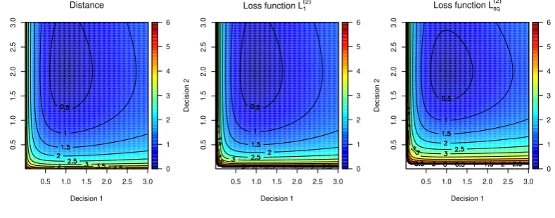
The comparison of loss functions
L
(2)1,
L
(2)sqand
D
+(2)for different values of decision
d
1and
d
2and fixed
θ
= (1
,
2)
Tis given in Figure 1.
0.5 1.0 1.5 2.0 2.5 3.0
0.5 1.0 1.5 2.0 2.5 3.0 Distance Decision 1 Decision 2 0 1 2 3 4 5 6
0.5 1.0 1.5 2.0 2.5 3.0
0.5 1.0 1.5 2.0 2.5 3.0
Loss function L1
(2)
Decision 1 Decision 2 0 1 2 3 4 5 6
0.5 1.0 1.5 2.0 2.5 3.0
0.5 1.0 1.5 2.0 2.5 3.0
Loss function Lsq
(2)
[image:12.595.101.496.381.536.2]Decision 1 Decision 2 0 1 2 3 4 5 6
Figure 1. Contour plots of loss functionsD(2)+ ,L(2)1 ,L
(2)
sq for the casem= 2 andθ= (1,2)T.
The proposed loss functions perform similar to the distance
D
(2)+, but have some
more favourable properties, like convexity.
5. Examples
Below, we investigate the performance of the proposed loss function and
correspond-ing Bayes estimators in more general settcorrespond-ings. We consider four classic examples of
estimation to demonstrate the essential differences of estimators. We focus on the
small sample size (
n
= 15) to emphasize the difference in estimators. The results for
moderate (
n
= 100) and large (
n
= 1000) sample sizes are given in Supplementary
Materials.
For all examples, the frequentist operating characteristic, Mean Squared Error
(MSE), is chosen to compare the different estimators on common grounds. As
ad-vocated by [3, 6], studying the frequentist properties of Bayes estimators is a way to
study the properties independently of the prior distribution and to consider Bayesian
point estimate simply as a function of the data. Furthermore, as we intend to
com-pare several Bayes estimators, which minimise different loss functions, the frequentist
characteristics are chosen to assess the performance of these estimators on an equal
basis. Note that this choice is not favourable to our new proposals, since the MSE is
derived from squared error loss.
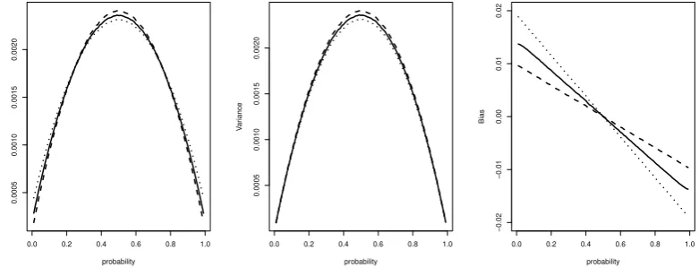
5.1. Estimation of a Probability
An important example of a parameter defined on the finite interval [0
,
1] is a
prob-ability. In the presence of a binary random sample with an unknown probability of
success a uniform distribution, i.e. a Beta prior distribution
B
(1
,
1) is often assumed,
a proposal which dates back to Laplace. Having observed
x
successes out of
n
trials,
the posterior distribution is a conjugate Beta distribution
B
(
x
+ 1
, n
−
x
+ 1). The
esti-mator corresponding to the squared error loss function (posterior mean) has the form
ˆ
p
q=
nx+1+2.
Another widely used estimator is the so-called “add two successes and two
failures” Agresti-Coull estimator [1] ˆ
p
AC=
xn+2+4.
Below we compare these approaches
to the newly proposed estimator (14).
The symmetric optimal Bayes estimator (14) in the case
a
= 0 and
b
= 1 can be
written
ˆ
diq
=
E
(
θ
2)
−
p
E
(
θ
2)(1
−
2
E
(
θ
) +
E
(
θ
2))
2
E
(
θ
)
−
1
where
θ
is a probability of success lying in the interval (0,1), over which a posterior
distribution is given. It is assumed that the extremes of the interval are not possible
values for the parameter. The first and second moments of a Beta distribution can
be computed explicitly and plugged in formula (14) to obtain the following interval
symmetric optimal Bayes estimator
ˆ
p
iq=
1 +
s
(
n
−
x
+ 1)(
n
−
x
+ 2)
(
x
+ 1)(
x
+ 2)
!
−1.
(18)
Simulated trials with sample size
n
= 15 are considered. On a grid of values
θ
∈
estimates found for each method. Then, the MSE is computed as
M SE
k≡
1
N
N
X
i=1
(ˆ
p
(ki)−
θ
)
2,
(19)
where ˆ
p
(ki)is a corresponding value in the
i
thsimulation and
k
=
q, iq, AC
corresponds
to an estimation method. The results are given in Figure 2.
0.0 0.2 0.4 0.6 0.8 1.0
0.004
0.008
0.012
probability
MSE
0.0 0.2 0.4 0.6 0.8 1.0
0.002
0.006
0.010
probability
V
ar
iance
0.0 0.2 0.4 0.6 0.8 1.0
−0.10
0.00
0.05
0.10
probability
[image:14.595.120.495.195.314.2]Bias
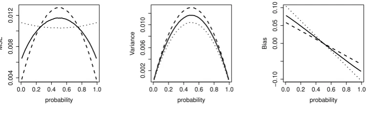
Figure 2. MSE, variance and bias for the restricted symmetric squared error loss function estimator ˆpiq
(solid), the squared error loss function estimator ˆpq (dashed) and the Agresti-Coull estimator ˆpAC (dotted).
Results are based onn= 15 observations and 109simulations.
The proposed estimator ˆ
piq
outperforms (in terms of the MSE) the Bayes estimator
obtained using the squared error loss function ˆ
p
qin the interval
θ
∈
(0
.
2
,
0
.
8). The cost
of this advantage is the worse performance on the intervals close to the bounds as the
proposed form of the loss function penalizes boundary decisions and by that drives
the final estimate away from them. However, the proposed estimator outperforms the
Agresti-Coull estimator ˆ
pAC
at the same intervals
θ
∈
(0
,
0
.
2) and
θ
∈
(0
.
8
,
1). Thus,
the proposed estimator might be considered as a trade-off between currently used
estimators ˆ
pq
and ˆ
pAC
, that outperforms ˆ
pAC
on bounds and ˆ
pq
away from bounds.
In addition to the MSE, the associated confidence intervals and coverage
probabil-ities are extensively studied in the literature [see e.g. 5]. In particular, coverage
prob-abilities were shown to have an erratic behaviour and often to go below their nominal
level. Corrections were proposed by [1]. Confidence intervals can also be constructed
around our newly proposed point estimator ˆ
piq
. The following confidence intervals are
compared via simulated coverage probabilities in Figure 3:
[1] Normal approximation confidence interval centred around ˆ
p
k,
k
=
q, iq, AC
as
suggested by [5]
CI
N(k)= ˆ
p
k±
z
α2
r
ˆ
p
k(1
−
p
ˆ
k)
n
,
where 1
−
α
is the confidence level.
[2] Wilson confidence interval centred around ˆ
p
AC[32]
CI
W(AC)=
x
+ 2
n
+ 4
±
2
√
n
n
+ 2
r
x
(
n
−
x
)
n
2+
[3] Approximate confidence interval using the delta-method centred around the
newly proposed ˆ
p
iqCI
D(iq)= ˆ
piq
±
2
q
ˆ
Viq
,
Viq
ˆ
=
∂f
(
x
)
∂x
2[image:15.595.97.498.108.365.2]
x=npiqˆ
n
piq
ˆ
(1
−
piq
ˆ
)
, f
(
x
) = ˆ
piq
.
Figure 3. Left panel: Coverage probabilities ofCIN(iq)(blue line),CIN(q)(red line) andCIN(AC)(purple line)
using [1], the normal approximation interval. Right panel: Coverage probabilities of CID(iq) (blue line) and CIW(AC)(purple line) using [2], the Wilson, and [3], the delta-method, confidence intervals respectively. Results are based onn= 15 observations and 109 simulations.
Using the normal approximation confidence interval, the coverage probability of
CI
N(q)goes below the nominal value for several values of
θ
. The coverage probabilities
of
CI
N(iq)and
CI
N(AC)also fluctuate but do not go below 0
.
95 for
N
= 15, which is
a desirable property. While one can find combination of
N
and
θ
for which coverage
probabilities
CI
N(iq)and
CI
N(AC)might be below 0
.
95 [5], it would be generally true that
their coverage probabilities are greater than of
CI
N(q)for larger intervals of
θ
and are
more robust. In addition, a comparison between the normal approximation method
(left panel of Figure 3) and the Wilson and delta method intervals (right panel of
Figure 3) supports the suggestion by [5] that the normal approximation method gives
a portmanteau way to construct simple confidence intervals with - on average - better
coverage probabilities than more complicated methods.
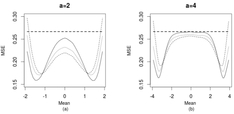
5.2. Restricted Estimation of a Normal Distribution Mean
In the following example, it is demonstrated what benefits the proposed form of loss
function (13) can provide in a Bayesian framework in the presence of the additional
information that the true parameter lies in an interval (
a, b
).
we refer the reader to [21] and for some recent generalizations to [20]. Interestingly,
despite the variety of the literature on the problem and the fact that the Bayes
esti-mator with respect to the uniform prior distribution on (
−
a, a
) outperforms uniformly
the “unrestricted” Bayes estimator under squared error loss function [10], the sample
mean estimator is still widely used in practice. For this reason, we propose our simple
alternative and compare it to the most commonly used estimators.
Consider the problem of estimating the mean
µ
of a normal sample of i.i.d.
X
i∼
N
(
µ, σ
2),
i
= 1
, . . . , n
where
σ
2is known. Assume it is known that the parameter
µ
belongs to the interval (
−
a,
+
a
) where
a >
0. A possible example is the estimation
of the treatment effect in paediatric studies of a clinical treatment that was already
tested on adults. An investigator might be sure that the same dosage of the drug as
given to adults would cause a greater level of toxicity in children. It is of interest how
much one can gain by incorporating this information in the estimator (14) compared
to currently used approaches that use the squared error loss.
As stated above, the common way to incorporate this information in a Bayesian
framework is restricting the prior distribution for the parameter of interest
µ
to the
interval (
−
a,
+
a
) and then using the squared error loss to obtain a point estimate (as
a summary of a posterior distribution). However, the information about the restricted
space is used only on the prior and ignored when choosing summary statistics, while
the proposed form of loss function (13) allows to incorporate it again. Moreover, in
practice the prior information is often ignored and the sample mean estimator
(cor-responding to Jeffrey’s prior) is used. Therefore, a comparison of the proposed loss
function and the currently utilized approaches (with and without the incorporation
the prior information) is of interest.
Consider samples of size
n
= 15 and alternative Bayes estimators as follows:
•
Bayes estimator under Jeffrey’s prior
g
(
µ
)
∝
k
p
nσ2
for
µ
and the squared error
loss function. Denoted by
J
;
•
Bayes estimator under the uniform prior
U
∼
(
−
a,
+
a
) for
µ
and squared error
loss function. Denoted by
U
1.
•
Bayes estimator (14) under the uniform prior
U
(
−
a,
+
a
) for
µ
and the interval
symmetric squared error loss function. Denoted by
U
2.Alternatively to
U
2, the Bayes estimatorU
20defined by (14), but with a wider interval
(
−
1
.
25
a,
+1
.
25
a
) is also applied to investigate how a lower penalization of the bounds
influences the estimation. This wider interval could be considered as a conservative
way to incorporate information about the location of the parameter.
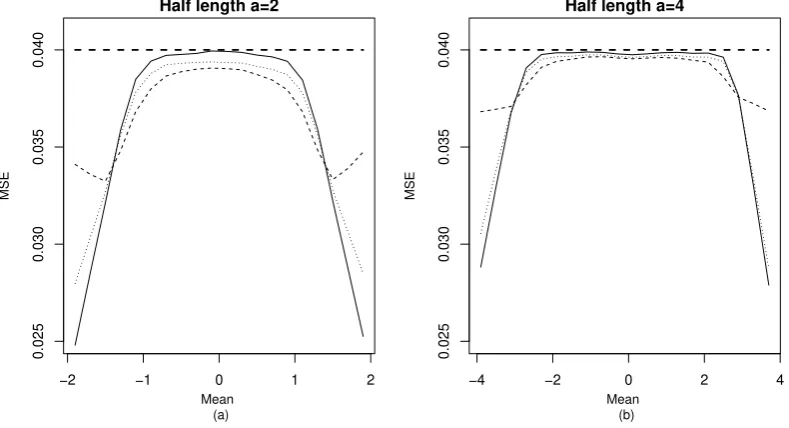
Two cases
a
= 2 and
a
= 4 are considered. The parameter
σ
2= 4 is assumed to be
known in both cases. As before, the
M SE
is used for a fair comparison of methods.
The results for 10
6replications for each value of
µ
are given in Figure 4.
Figure 4. MSE corresponding to different values of the restricted mean parameterµwith (a)a= 2 and (b) a= 4 and the Bayes estimatorU1 (solid),U2 (dashed) andU20 (dotted) and simple mean estimatorJ (solid
dashed). Results are based on 106 replications.
recommended for the application if boundary decisions lead to severe consequences.
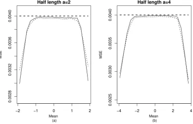
5.3. Bayesian Estimation of the Parameters of a Gamma Distribution
An important example of multidimensional restricted parameter estimation is a
Gamma distribution with positive shape and scale parameters
α
1, α
2>
0. Bayesian
inference for this problem has been studied, for example, in [23] and methods for
approximate computation of Bayes estimators were proposed using the Lindley
ap-proximation [18].
We consider the function
L
(2)sqgiven in (17) to obtain Bayes estimators. As the
loss function (17) is the sum of the univariate precautionary loss functions (2), the
following estimators are used ˆ
α
i=
p
E
(
α
2i)
, i
= 1
,
2 where the expectation
E
is taken
with respect to the posterior distribution.
Let us consider an experiment with sample size
n
= 15. The parameters of the
Gamma distribution are varied over a grid,
α
1, α
2∈
(0
,
10) and the performance of the
different approaches are compared by simulations. The two approaches compared use
the same prior distribution for parameters
α
1and
α
2using the following estimators:
1) Bayes estimator under the squared error loss function,
2) Bayes estimator under the multivariate precautionary loss function.
We use the same weakly informative Gamma prior distributions Γ(10
−4,
10
−4) of
(
α
1, α
2) with parameters for both estimation methods and an approximate method
proposed by [18]. The weakly informative distribution are chosen to minimise the
influence of the prior distribution on the comparison of estimators and corresponds to
the situations of no prior knowledge about the parameters. We would like to emphasize
that the choice of the prior distribution is out of the scope of this paper and the goal is
to compare two Bayes estimators when all other parameters are equal. The difference
between the MSE of estimators based on method (1 against method 2) for parameters
α
1and
α
2in 10
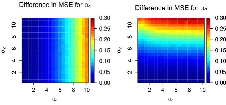
9simulations is given in Figure 5.
2 4 6 8 10
2
4
6
8
10
Difference in MSE for
α
1α1
α
2
0.00 0.05 0.10 0.15 0.20 0.25 0.30
2 4 6 8 10
2
4
6
8
10
Difference in MSE for
α
2α1
α
2
[image:18.595.93.489.80.265.2]0.00 0.05 0.10 0.15 0.20 0.25 0.30
Figure 5. Difference in the MSEs for parametersα1 andα2 for their different true values and using Bayes
estimator under the squared error loss function and Bayes estimator underL(2)sq. Results are based on 109
replications.
parameters
α
1and
α
2. It means that the Bayes estimator from method 2) is associatedwith smaller MSE than the Bayes estimator from method 1). The difference in the
MSE increases as the true value of the parameter increases. This result makes the
proposed estimator and the associated loss function
L
(2)sqgood candidates for further
investigation in multidimensional estimation problems.
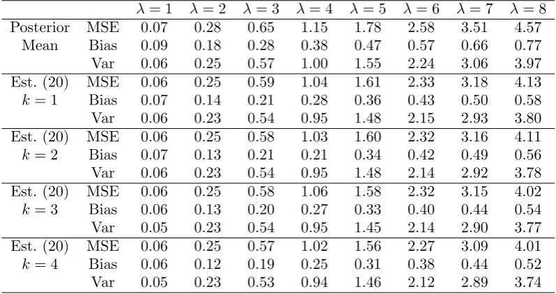
5.4. Bayesian Estimation of the Parameters of a Weibull Distribution
Another important example of multidimensional restricted parameters estimation is
the Weibull distribution which positive scale and shape parameters
λ, ν >
0. The
Weibull distribution is of great importance in applications as it is widely employed in,
for example, reliability engineering, extreme value theory and survival analysis [26].
Bayesian inference for this problem has been studied in [9]. Importantly, despite both
parameters being defined on the positive real line only, the squared error loss function
(and associated posterior mean Bayes estimator) are used in these works. Below, we
consider how the novel loss function (7) and the associated Bayes estimator behaves
in this estimation problem.
We consider the function
L
(km)given in (16) to obtain Bayes estimators. As the loss
function (16) is the sum of the univariate loss functions (6), the following Bayesian
estimators are used for both scale parameters of Weibull distribution
ˆ
λk
=
E
(
λ
k)
E
(
λ
−k)
1/2k,
νk
ˆ
=
E
(
ν
k)
E
(
ν
−k)
1/2k(20)
where the expectations are taken with respect to the posterior density function. Note
that the estimators depend on the parameter of the loss function
k
. We will investigate
the influence of the parameter on the estimation.
{
(0
.
5
,
1
,
5
,
10
,
15)
}
, and the performance of different approaches are compared by
simu-lations. Again, the two approaches compared use the same weakly information Gamma
prior distribution Γ(10
−4,
10
−4) for both positive parameters, as we would like to
min-imise the impact of the prior distribution on the comparison.
We start from the comparison of
1) Bayes estimators under the squared error loss function,
2) Bayes estimators (20) under the multivariate
L
(1m)(16) for
k
= 1.
The difference between the MSE of estimators (method 1 against method 2) for positive
parameters
λ
,
ν
in 10
4simulations are given in Table 1. The MSE for
ν
are scaled by
1
[image:19.595.170.426.266.412.2]νλ
to obtain the results on a similar scale for various parameters.
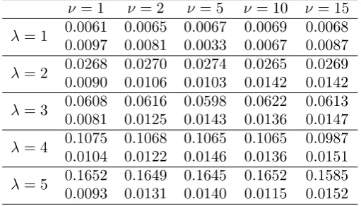
Table 1. Difference in the MSEs for parameters λ(upper lines) andν (lower lines) for their different true
values and using Bayes estimator under the squared error loss function and Bayes estimator underL(1m). Results are based on 104 replications.
ν
= 1
ν
= 2
ν
= 5
ν
= 10
ν
= 15
λ
= 1
0.0061
0.0065
0.0067
0.0069
0.0068
0.0097
0.0081
0.0033
0.0067
0.0087
λ
= 2
0.0268
0.0270
0.0274
0.0265
0.0269
0.0090
0.0106
0.0103
0.0142
0.0142
λ
= 3
0.0608
0.0616
0.0598
0.0622
0.0613
0.0081
0.0125
0.0143
0.0136
0.0147
λ
= 4
0.1075
0.1068
0.1065
0.1065
0.0987
0.0104
0.0122
0.0146
0.0136
0.0151
λ
= 5
0.1652
0.1649
0.1645
0.1652
0.1585
0.0093
0.0131
0.0140
0.0115
0.0152
The differences in the MSEs for both parameters are positive for all considered
true values of
λ
and
ν
. It follows that the Bayes estimator from method 2) leads to a
smaller MSE than the estimator corresponding to the squared error loss function. For
a fixed value of
ν
, the MSE corresponding to
λ
increases with the parameters. The
scaled MSE corresponding to
ν
stays nearly the same for various values of
λ
. Overall,
the proposed estimator and the associated loss function can be good candidates to be
used for the parameters defined on the positive real line.
Table 2. MSE, Bias and Variance for the Bayes estimator ofλ∈(1,8) corresponding to the squared error loss function (posterior mean) and for the estimator ˆλk given in Equation (20) fork= 1,2,3,4. Results are
based on 104 replications.
![Figure 3.Left panel: Coverage probabilities ofusing [1], the normal approximation interval](https://thumb-us.123doks.com/thumbv2/123dok_us/9304214.431697/15.595.97.498.108.365/figure-left-coverage-probabilities-ofusing-normal-approximation-interval.webp)