Face Detection with Boosted Gaussian Features

(1)

www.elsevier.com/locate/pr

Face detection with boosted Gaussian features

Julien Meynet

a,∗

_{, Vlad Popovici}

b

_{, Jean-Philippe Thiran}

a

a_{Ecole Polytechnique Fédérale de Lausanne (EPFL), Signal Processing Institute, CH-1015 Lausanne, Switzerland} b_{Bioinformatics Core Facility, Swiss Institute of Bioinformatics, CH-1015 Lausanne, Switzerland}

Received 7 April 2006; received in revised form 21 December 2006; accepted 7 February 2007

Abstract

Detecting faces in images is a key step in numerous computer vision applications, such as face recognition or facial expression analysis. Automatic face detection is a difficult task because of the large face intra-class variability which is due to the important influence of the environmental conditions on the face appearance. We propose new features based on anisotropic Gaussian filters for detecting frontal faces in complex images. The performances of our face detector based on these new features have been evaluated on reference test sets, and clearly show improvements compared to the state-of-the-art.

Keywords:Face detection; AdaBoost; Gaussian features

1. Introduction

Automatic face detection is a key step in any face processing system. Its goal is to detect the presence of human faces in a still image and to return their position (which may be given in terms of a bounding box for example). The performance of latter stages of processing (e.g. face recognition, face authentication or facial expression recognition) is conditioned by the quality of the detection[1]. However, automatic detection of faces is far from being a trivial task. Its complexity is due to the large intra-class variability, as faces are highly deformable objects whose appearance depends on numerous factors (lighting conditions, presence or absence of occluding objects, etc.). Moreover, in most face detection systems, it is necessary to model also the “non-face” class, which proves to be very difﬁcult.

In the last years, many methods have been proposed and we give hereafter a brief overview of some of the most signiﬁ-cant ones. There are two main approaches for detecting faces: holistic methods which consider the face as a global object and

∗_{Corresponding author. Tel.: +41 21 6933632; fax: +41 21 6937600.}

E-mail addresses:Julien.Meynet@epﬂ.ch(J. Meynet),

[email protected](V. Popovici),JP.Thiran@epﬂ.ch(J.-P. Thiran) URLs:http://itswww.epﬂ.ch/∼meynet(J. Meynet),

http://www.isrec.isb-sib.ch/∼vpopovic(V. Popovici), http://itswww.epﬂ.ch/∼thiran(J.-P. Thiran).

feature-based methods which try to recognize parts of the face and assemble them to take the final decision. Other techniques can also use a mix of both approaches. The first category usually produces very fast detectors with better classification perfor-mances and turns out to be more robust to light changes. How-ever, one of the main advantages of the feature-based methods is that they are more robust to head pose changes. In this work we only consider frontal faces and thus, in the remaining of the paper, only the holistic methods will be considered. More detailed surveys are given in Refs.[2,3].

The classical approach for face detection is to scan the input image with a sliding window and for each position, the win-dow is classified as either face or non-face. The method can be applied at different scales (and possibly different orientations) for detecting faces of various sizes (and orientations). Finally, after the whole search space has been explored, an arbitration technique may be employed for eliminating multiple detections. Of course the efficient exploration of the search space is a key ingredient for obtaining a fast face detector. There are various methods for speeding up this search, like using additional in-formation (e.g. skin color) or using a coarse-to-fine approach. Nevertheless the most important component of the system is the classifier deciding whether a given window contains a face or not. From this perspective, this paper focuses on both aspects, efficient search space and robust classifier.

(2)

to detect faces at any scale and position they use a sliding window which scans a pyramid of images at different scales. A similar holistic approach proposed by Rowley et al.[5] is one of the most representative for the class of neural network approaches. It comprises two modules: a classification module which hypothesizes the presence of a face and a module for arbitrating multiple detections. A fast algorithm is proposed by Viola and Jones[6]. It is based on three main ideas. They first train a strong classifier by boosting the performance of simple rectangular Haar-like features-based classifiers. They use the so-called integral image as image representation which allows to compute the base classifiers very efficiently. Finally they introduce a classification structure in cascade in order to improve both the detection speed and the classification results. This last method (in particular the cascade structure) leads to a very fast detection (about 30 frames per second on a standard PC for 320×240 images). As it will be explained later in the paper, we have used this method as a pre-processing step in order to reduce the search space.

In this work we present anisotropic Gaussian filters (GF) that model efficiently the face appearance. As we will show, these local filters present the advantage of being more discrimina-tive than the Haar-like features introduced in Ref.[6], while remaining simple to compute, and thus compatible with real time implementation.

The remaining of the paper is structured as follows. Section 2 introduces the new geometrical ﬁlters and discusses their ability to model the face patterns. It also gives a brief overview of AdaBoost, a learning algorithm that selects iteratively the best features. Section 3 reports some results as well as comparisons with relevant existing face detectors. Finally, we draw some conclusions and explain the future work in Section 4.

2. Boosted anisotropic Gaussian features 2.1. AdaBoost

Training a statistical face detector consists in learning a model from a set of face and non-face patterns. This section explains how we build this model using a learning algorithm called AdaBoost (for Adaptive Boosting). AdaBoost was pro-posed in 1995 by Freund and Schapire[7]as an efficient algo-rithm of the ensemble learning field. It is a greedy algoalgo-rithm which constructs an additive combination of weak classifiers such that it minimizes the exponential loss:

L(y, f (x))=exp(−yf (x)), (1) wherexif the pattern to be classiﬁed,yits target label andf (x) the decision function which outputs the decided class label. AdaBoost combines iteratively the weak classiﬁers by taking into account a weight distribution on the training samples such

Freund and Schapire [7] showed that the generalization error

Ris bounded by RP[yf_T(x)] +O d N2 ∀>0, (2)

where fT is the decision function output by AdaBoost, d is

theVC-dimensiondeﬁned by Vapnik[8] andNis the number

of examples. This bound in Eq. (2) is quite loose but it shows that larger margins lead to smaller upper bounds on the testing error. Like many other learning algorithms, AdaBoost has an important drawback: it tends to overﬁt training samples when they are noisy. The inﬂuence of the noisy samples will be discussed in Section 2.4.

Note that depending on the application we might prefer de-tecting all the faces and accept more false alarms than taking an equal error rate. In AdaBoost, this can be easily implemented by building an asymmetric version of AdaBoost that encour-ages the correct classiﬁcation of the positive examples. This can be done for example by penalizing the negative examples in the initial sample weight distribution. The ﬁnal threshold is also tuned on an independent validation set in order to obtain the desired operating point on the ROC curve.

2.2. Anisotropic Gaussian ﬁlters

In this section we propose a new set of local filters to be used for constructing the weak classifiers. The filters are made by a combination of a Gaussian in one direction and its first derivative in the orthogonal direction.

These functions have been introduced by Peotta et al.[9]for image compression and signal approximation. The generating function(x, y):R2→Ris given by

(x, y)=xexp(−|x| −y2). (3) It efﬁciently captures contour singularities with a smooth low resolution function in the direction of the contour and it ap-proximates the edge transition in the orthogonal direction with the ﬁrst derivative of the Gaussian.

In order to generate a collection of local ﬁlters, the following transformations can be applied to the generating function: (1) Translation by(x0, y0)

Tx0,y0(x, y)=(x−x0, y−y0). (2) Rotation by

(3)

Fig. 1. Anisotropic Gaussian ﬁlters with different rotating and bending pa-rameters. (3) Bending byr Br(x, y)= ⎧ ⎪ ⎪ ⎪ ⎪ ⎪ ⎪ ⎨ ⎪ ⎪ ⎪ ⎪ ⎪ ⎪ ⎩ r− (x−r)2+y2_, _if_{x < r,} rarctan y r−x r− |y|, x−r+r 2 ifxr. (4) Anisotropic scaling by(sx, sy)

Ssx,sy(x, y)= x sx, y sy .

By combining these four basic transformations, we obtain a large collection of functions:

_i(x, y)=_s_x_,s_y_,_,r,x0,y0(x, y) (4) =Tx0,y0RBrSsx,sy(x, y). (5) DenoteDthis collection.Fig. 1shows some of these functions with various bending and rotating parameters.

At each iteration of AdaBoost, a weak learner is called to train simple classifiers from the collection of geometrical filters. Many techniques can be used to train these weak classifiers. The simplest weak learner consists in learning a threshold and a parity for each filter response. More sophisticated constructions were proposed by Lienhart et al.[10]. They proposed CART trees which allow to learn dependencies between the features. However, equivalent results can be obtained using the simple classifiers by adding few more iterations in AdaBoost. More-over, AdaBoost only requires classifiers that are slightly better than random guessing so this choice will not affect significantly the convergence of the learning.

We thus consider a simple linear classifierhj :R→ {−1,1} for each filter configuration by choosing two parameters: a threshold_jand a paritypj as shown in Eq. (6). These param-eters are chosen using the Bayes decision rule.

hj(x)=

1 if pjfj(x) < pjj,

−1 otherwise, (6)

where the feature fj(x) is the scalar product between the image and the ﬁlter _j corresponding to a particular ﬁlter

Fig. 2. Some of the ﬁrst selected base functions.

Fig. 3. Haar-like templates.

conﬁguration(sx, sy,, r, x0, y0): ∀_j ∈D fj(x)=

X×Yj(x, y)I (x, y)dxdy. (7)

Fig. 2 shows some functions selected in the ﬁrst iterations of AdaBoost. It turns out that they are particularly well adapted to capture local contours that are insensitive to changes of the lighting conditions. In comparison, Haar ﬁlters[6]model global contrasts that are more sensitive the direction of the light source.

2.3. Gaussian vs. Haar-like

This section shows a comparison between the Haar-like ﬁl-ters (HF) proposed in Ref.[6]and the anisotropic GF described above.

The HF are made of 2, 3 or 4 rectangular masks and have four parameters: horizontal and vertical scaling and the coordi-nates of the center. The templates are shown inFig. 3. A very important advantage of the HF is that they can be computed extremely efﬁciently using a so-called integral image represen-tation.

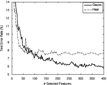
To give a quantitative comparison between HF and GF, two boosted classiﬁers have been trained on the same training set containing face and non-face images using AdaBoost algorithm described in Section 2.1. The results are evaluated on a large validation set extracted from some reference datasets (see Sec-tion 3).Fig. 4gives a comparison of the intrinsic performances of each feature type. The test error decreases quickly with the number of AdaBoost iterations but it stops decreasing after roughly 100 iterations in the case of HF while it keeps decreas-ing with GF. Intuitively, after several iterations, AdaBoost fo-cuses on the hard to classify examples and the simplistic HF are not discriminant enough to separate the two classes. The bet-ter performances of the Gaussian features also clearly appear in the receiver operating characteristic (ROC) analysis (Fig.5). The ROC curves are drawn by changing the threshold of the ﬁnal decision output by AdaBoost.

Let us now evaluate the time needed for computing each feature. We trained two similar classiﬁers with 200 HF on one hand and 200 GF on the other hand. By applying these two

(4)

Fig. 4. Performance of GF and HF-based detectors on a test set.

Fig. 5. ROC curves for Gaussian and Haar-like features.

classiﬁers on several images, we compared the average compu-tation time for applying a single HF and a single GF. We found that computing a GF takes in average 2.86 more time than a HF. (Note that the GF are precomputed in the model such that the expensive computation of the generative function is avoided.)

An interesting point to notice here is the shape of the GF that are selected by AdaBoost (Fig.2). The ﬁrst functions chosen have generally large scale parameters, they can globally model the face appearance whereas more local features are extracted later in the selection process.

HF are only binary ﬁlters, thus they may be able to well capture the contrast between image regions but will be limited for modeling smooth transitions present in facial images. GF are continuous functions more appropriate to model continu-ous natural images. The ﬂexibility due to the large number of parameters allows to model contour singularities as well as in-tensity changes in large regions (with large scaling parameters).

Fig. 6. Reduction of the search space by a simple cascade of Haar features.

2.4. Cascade of classiﬁers

In order to speed up the scanning process, cascades of classi-fiers are used instead of using directly a strong classifier trained on the complete training set. A cascade is a sequential combi-nation of classifiers where each stage is tuned to work in a pre-defined regime (by choosing an operating point on the ROC). If an example is rejected at any stage of the cascade it will be rejected by the global classifier and there is no need of process-ing further stages. The advantage of usprocess-ing a cascade instead of a single classifier is the following: it speeds up the decision process by only applying simple classifiers to candidates easy to discard while keeping the most complicated and time con-suming stages for the challenging examples. Moreover, training each stage of the cascade on different subsets of the training set reduces the risk of overtraining the data as described in Section 2.1 by reducing the influence of potential outliers.

In Fig. 4 we can see that Haar-like features are compara-tively efficient for building the first linear classifiers. In or-der to use their computation efficiency (especially if they are computed using the integral image trick (see Ref.[6])), a sim-ple five staged cascade of Haar-like features is added as a pre-processing to our final Gaussian-based classifier. This effi-ciently reduces the search space such that only few remaining windows need to be tested with the Gaussian models. Fig. 6

gives the average percentage of negative windows discarded by each of these ﬁve ﬁrst stages on the CMU/MIT test set[11]. Numerical results about the speed of the detector will be given in Section 3.4.

3. Experiments and results 3.1. Structure of the system

In order to measure the performances of this system and com-pare it with other relevant methods the following experiments

(5)

Fig. 7. Results on images of BANCA[16]in the complex adverse scenario.

have been performed. First of all, a 20×15 pixels window is used to scan the images. It is then dilated by powers of 1.2 in order to detect faces at different scales. A very simple arbitra-tion method clusters the neighbor positive windows such that only one detection per face is returned. This is done by keeping the median window for each cluster.

For training the models, face images were collected from some classical face datasets: XM2VTS [12], BioID [13], FERET[14]. After adding some variations in scale, in-plane rotations and shifts, the complete face training set contained 9500 images. The non-face dataset was bootstrapped from randomly selected images without human faces. A total of roughly 500 000 non-face images were ﬁnally used. These two datasets are available upon request.

Before training we had to choose the parameters of the trans-formations to be applied to the HF and GF. These transforma-tions would then condition the size of the setDof filters and, consequently, the dimensionality of the feature space. The set of HF that we used to train the cascade contained 37 520 fil-ters (all possible combinations in a 20×15 pixels window). In the case of GF, considering all the possible combinations of the six filter parameters would produce a huge set of filters. We thus decided to subsample the complete set of filters in order to keep a manageable set for the training process. For this, we noticed that slight variations of the two scaling parameters and the rotation parameter do not change significantly the response of the filter. The other three parameters are more unstable in the sense that small changes may have large effects on the re-sponse of the filter. The parameter space has been subsampled according to these previous remarks. The final set of GF that we used for training the classifiers contains 202 200 features. This set of GF gives a good trade-off between training com-plexity and parameter flexibility.

An ambiguous point in face detection algorithms is the way the performances are measured. Papers usually provide the detection rate and the false positive rate to show the quality of their system; however, they often consider different measures for those rates. It appears to be very difﬁcult to objectively com-pare different published results. In this work, the problem is addressed using the evaluation protocol proposed by Popovici et al.[15]. The evaluation is performed by taking into account

Table 1

Comparisons of various methods tested on the BANCA[16]data base

Classiﬁer % of detections

with score>0.95 (following Ref.[15])

Five stages Boosted HF 52.08

12 Stages Boosted HF 86.78

12 Stages Boosted GF 91.02

Five stages Boosted HF + 12 stages Boosted GF

90.74

Results are reported for the French and English parts following the evaluation protocol described in Ref.[15]. Detections with a global score larger than 0.95 are considered as correct.

several parameters between the detected location and the ground-truth annotated positions. The scoring function mea-sures the ratio of the between-eyes distances, the angle between the eyes axis and of course the distance between the annotated and detected eye positions. This method gives a more objec-tive scoring of the detection performances. See Ref. [15] for details on how to use the scoring function.

3.2. BANCA data base

The system has been tested on two distinct datasets. On the one hand we considered the BANCA data base[16]which was built for training and testing multi-modal veriﬁcation systems. The face images were acquired using various cameras and un-der several scenarios (controlled, degraded and adverse). Some examples of detection results of the adverse scenario are shown in Fig. 7. In this work, we used 12 480 images from the so-called French and English datasets as we dispose of precise groundtruth annotations for these ones.

Table 1 gives a comparison of four variants of the system tested on the BANCA data base. We first tested five stages of HF to evaluate the efficiency of the few first features selected. Then a complete cascade of 12 stages of HF is compared to the same structure using GF. Finally we tested a GF cascade preprocessed by the five first stages of a HF cascade. First of all it confirms that a cascade trained with GF gives much better detection rates than using HF. Then it is interesting to

(6)

Fig. 8. Detection scores using the evaluation protocol[15]including the two individual scores (shift and scale) and the global score. Note that a logarithmic scale is used.

Table 2

Performances on the CMU/MIT test set[11]

Methods Dataset 1 Dataset 2 Dataset 3

D.R. (%) F.A. D.R. (%) F.A. D.R. (%) F.A.

Rowley et al.[5] 87.1 15 92.5 862 90.5 570

Sung and Poggio[4] 81.9 13 — — — —

Shneiderman and Kanade[17] — — 93.0 88 94.4 65

Viola and Jones[6] — — — — 91.4 50

12 Stages HF 83.7 20 88.6 95 88.3 50

Five stages HF + 12 stages GF 88.3 17 92.8 88 91.7 50

Three datasets conﬁgurations are considered: Dataset 1: 155 faces, Dataset 2: 483 faces, Dataset 3: 507 faces. It shows the Detection rate (D.R.) and number of false alarms (F.A.) for each method.

notice that a very simple preprocessing by a ﬁve staged cascade of HF followed by a Gaussian based model does not affect signiﬁcantly the performances compared to GF alone. We thus

can benefit from the computation efficiency of the HF without decreasing the detection rate and then take advantages of the GF discrimination to improve the classifier accuracy.

(7)

The evaluation protocol [15] allows to measure the main characteristics of our detector. Each individual criterion in

Fig. 8shows that when a face is correctly detected, the bound-ing box returned by the detector is really precise both in scale and shift (and of course also in angle as we only test upright faces). However, there is a bit more imprecision with respect to the shift score. This can be explained by the trivial arbitra-tion criterion that we use for merging the multiple detecarbitra-tions around each face.

3.3. CMU/MIT test set

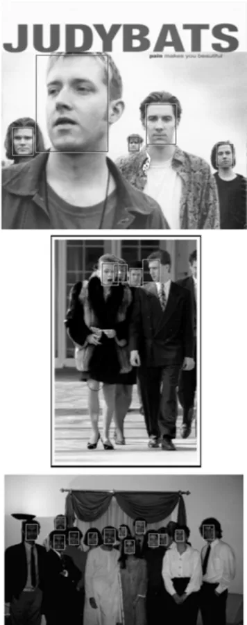
We now consider a more challenging data base commonly used to evaluate performances of face detectors especially on very low resolution faces. The CMU/MIT Test set [11] was ﬁrst introduced by Rowley [5] for testing. The ﬁrst version of this test set contained 23 images with a total of 155 very low resolution faces (it is referred as Dataset 1 in Table 2). The complete set contains 130 images with 507 faces (Dataset 3 in Table 2). However, some of these annotated faces are manually drawn and they are counted as false detections in some publications. To address this ambiguity, some papers only consider 123 images with 483 faces (Dataset 2 inTable 2). The three versions of the dataset are tested in this paper to avoid any confusion.Fig. 9shows some detection results on images of this data base.

Table 2gives comparisons with the state-of-the-art methods on these datasets. It gives global performances of two versions of the system: a cascade of HF and a cascade of GF prepro-cessed by ﬁve stages of HF. The results in this table have to be taken cautiously as they are affected by many factors: the scan-ning parameters (scaling factor, window shifting step, etc.), the technique chosen for merging overlapping windows, the num-ber of training patterns and so forth. In particular, the way the non-face training examples are generated has a great impact on the decision functions. Finally some systems used additional post-processing to improve the results. For example, Viola et al.[6] used a voting strategy between several cascades to re-duce the false positive rate. This explains why our cascade of HF has slightly lower performances than the implementation in Ref.[6]. However, the use of GF gives roughly similar results with Ref.[6]without any post-processing, especially since we used only 1260 features in our cascade instead of 6061 in Ref.

[6]. Shneiderman and Kanade[17]report good performances. However, they use several intensity corrections and a complex wavelets-based network that lead to extremely heavy computa-tion. It is clear that a face detector with our new features imple-mented with the pre-processing and post-processing strategies of the other methods would lead to a very performant system. But such an implementation is out of the scope of this paper.

The goal of this paper is to show the advantages of using the Gaussian filters compared to Haar-like filters. Therefore, a ROC is given inFig. 10. The two models were trained us-ing the same data and the evaluation is performed with strictly identical parameters. It shows that the use of the new filters brings an important improvement in term of detection

capabil-Fig. 9. Face detection results on some images of the MIT/CMU testset[11]. ities on real world data. For instance, considering a detection rate of 90% for both classiﬁers, there are twice less false alarms with GF.

(8)

Fig. 10. ROC analysis for comparing the algorithms on the MIT/CMU testset [11].

Table 3

Detection speed in frames per seconds (fps) of three detectors

Detector fps

12 Stages HF 28.63

12 Stages GF 17.69

5 Stages HF + 12 stages GF 27.32

The measure is an average over the 1500 frames of a sequence of 320×240 pixels images.

3.4. Processing speed

The drawback of the new filters is that the learning complex-ity is increased because of the larger number of candidate filters. It was also noted in Section 2.3 that computing the response of a GF was roughly three times more expensive than applying a Haar filter. However, we show in this section that the use of GF will not affect significantly the overall detection speed.

Let us consider again three detectors: 12 stages of HF, 12 stages of GF and 12 stages of GF pre-processed by ﬁve stages of HF. We apply these three detectors on a sequence of 1500 images with 320×240 pixels, each frame containing one or several faces. We then report inTable 3the average detection speed (number of frames per seconds) for the three detectors.

As expected, the detector with only GF is slower than the other detectors. However, a simple pre-processing by ﬁve stages of HF allows the detector to be only slightly slower than the complete cascade of HF. In fact the ﬁve stages of HF discard a large majority of non-face windows so that the computation of the GF does not affect much the overall detection speed.

4. Conclusions

This paper presents a new face detection system using Gaus-sian based ﬁlters which leads to high detection performances

combination of several parallel classiﬁers in order to reduce the false positive rate.

Acknowledgments

This work is supported by the Swiss National Science Foun-dation through the National Center of Competence in Research on “Interactive Multimodal Information Management (IM2)”. References

[1]Y. Rodriguez, F. Cardinaux, S. Bengio, J. Mariéthoz, Estimating the quality of face localization for face veriﬁcation, IEEE International Conference on Image Processing, ICIP, vol. 1, 2004, pp. 581–584. [2]E. Hjelmas, B.K. Low, Face detection: a survey, Comput. Vision Image

Understand. 83 (3) (2001) 236–274.

[3]N. Ahuja, M. Yang, D. Kriegman, Detecting faces in images: a survey, IEEE Trans. Pattern Anal. Mach. Intell. 24 (1) (2002) 34–58. [4]K.K. Sung, T. Poggio, Example-based learning for view-based human

face detection, IEEE Trans. Pattern Anal. Mach. Intell. 20 (1) (1998) 39–51.

[5]H.A. Rowley, S. Baluja, T. Kanade, Human face detection in visual scenes, in: D.S. Touretzky, M.C. Mozer, M.E. Hasselmo (Eds.), Advances in Neural Information Processing Systems, vol. 8, The MIT Press, Cambridge, MA, 1996, pp. 875–881.

[6]P. Viola, M.J. Jones, Robust real-time face detection, Int. J. Comput. Vision 57 (2) (2004) 137–154.

[7]Y. Freund, R.E. Schapire, A decision-theoretic generalization of on-line learning and an application to boosting, J. Comput. Syst. Sci. 55 (1) (1997) 119–139.

[8]V.N. Vapnik, The Nature of Statistical Learning Theory, Springer, New York, NY, USA, 1995.

[9]L. Peotta, L. Granai, P. Vandergheynst, Very low bit rate image coding using redundant dictionaries, in: Proceedings of the SPIE, Wavelets: Applications in Signal and Image Processing X, vol. 5207, SPIE, November 2003, pp. 228–239.

[10]R. Lienhart, A. Kuranov, V. Pisarevsky, Empirical Analysis of Detection Cascades of Boosted Classiﬁers for Rapid Object Detection, Lecture Notes in Computer Science, vol. 2781, 2003, pp. 297–304.

[11]H.A. Rowley, S. Baluja, T. Kanade, Neural network-based face detection, IEEE Trans. Pattern Anal. Mach. Intell. 20 (1) (1998) 23–38. [12]K. Messer, J. Matas, J. Kittler, J. Luettin, G. Maitre, Xm2vtsdb: the

extended m2vts database, in: Second International Conference on Audio and Video-based Biometric Person Authentication, 1999.

[13]R.W. Frischholz, U. Dieckmann, Bioid: a multimodal biometric identiﬁcation system, Computer 33 (2) (2000) 64–68.

[14]P.J. Phillips, et al., The FERET database and evaluation procedure for face-recognition algorithms, Image Vision Comput. 16 (1998). [15]V. Popovici, J. Thiran, Y. Rodriguez, S. Marcel, On performance

evaluation of face detection and localization algorithms, in: J. Kittler (Ed.), Proceedings of the 17th International Conference on Pattern Recognition, vol. 1, IEEE, New York, August 2004, pp. 313–317. [16]E. Bailly-Bailliere, et al., The banca database and evaluation protocol,

in: 4th International Conference on Audio- and Video-Based Biometric Person Authentication, Guildford, UK, Berlin, June 2003, Lecture Notes in Computer Science, vol. 2688, Springer, Berlin, 2003, pp. 625–638. [17]H. Schneiderman, T. Kanade, A statistical approach to 3D object

detection applied to faces and cars, in: International Conference on Computer Vision, 2000.

(9)

About the Author—JULIEN MEYNET is currently pursuing the Ph.D. degree at the Signal Processing Institute, Swiss Federal Institute of Technology (EPFL), Lausanne, Switzerland. He received his Engineering and M.Sc. degrees electrical engineering from the Grenoble Institute of Technology (INPG), Grenoble, France in 2003.

He has been at EPFL since 2003 as assistant researcher. His main current research interests include multiple classiﬁer systems and their applications in computer vision.

About the Author—VLAD POPOVICI is researcher with Swiss Institute of Bioinformatics (SIB), working on different theoretical and applied aspects of statistical pattern recognition. He has obtained his Engineering and M.Sc. degrees in computer science from Technical University of Cluj-Napoca, Romania, in 1998 and 1999, respectively, and his Ph.D. from Swiss Federal Institute of Technology (EPFL) in 2004. Before joining SIB he has worked for Digital Media Institute, Tampere University of Technology as research scientist and for Signal Processing Institute at EPFL as assistant researcher and, later, as post-doctoral researcher. His current research focusses on sparse classiﬁers and multiple classiﬁer systems, and their applications to life sciences.

About the Author—JEAN-PHILIPPE THIRAN was born in Namur, Belgium, in August 1970. He received the Electrical Engineering degree and the Ph.D. degree from the Université catholique de Louvain (UCL), Louvain-la-Neuve, Belgium, in 1993 and 1997, respectively.

Dr Thiran is the Assistant Professor and the leader of the Image Analysis Group at the Signal Processing Institute of the Swiss Federal Institute of Technology (EPFL), Lausanne, Switzerland. His current scientiﬁc interests include image segmentation, prior knowledge in image analysis, PDEs in image analysis, multimodal signal processing, medical image analysis, including multimodal image registration, segmentation, computer-assisted surgery, diffusion MRI, etc. Prof. Thiran is author or co-author of more than 50 journal papers and 90 conference papers on image analysis and owns of four international patents.