CHANNEL ESTIMATION AND MODELLING OF
MIMO IN INDOOR ENVIRONMENT
D. Sanjana1, D. Sarala2, D. Sridevi3, P Sai sree4, Dr Seetaiah Kilaru5
I.INTRODUCTION
I It is a well-known fact that the amount of information transported over communication systems grows rapidly. Not only the file sizes increase, but also bandwidth-hungry applications such as video on demand and video conferencing require increasing data rates to transfer the information in a reasonable amount of time or to establish real-time connections. To support this kind of services, broadband communication systems are required.
Another well-known fact is that the mobility of communication systems is more and more demanded. One example is the enormous increase of mobile phone users worldwide. Another example is the trend of the work place becoming increasingly mobile. A term often used in this context is office hotelling. Hotelling is a form of alternative officing in which employees who work out of the office for significant periods of time can call ahead (just as they do in making hotel reservations) and reserve workspace. They select an office from a specially-designated block of workspaces when they come into the company’s office facilities. This allows organizations to reduce space costs by relying on technology to create the appearance of a permanent office. Ideally, the employee should be completely mobile within the office, and still be able to connect his personal computer to the computer network. Thus, a wireless computer network is desirable.
Another place where wireless computer networking is in demand is at the university campus. A growing number of universities offer their students the possibility to buy a laptop from university. The way of teaching is adapted to the availability of laptops. To make this kind of studying efficient, students need to be able to connect to the computer network of the university in order to download the study material that the professor offers. However, it is undoable to adapt the computer network infrastructure in such a way that the students can plug-in in every (lecture-) room at the university. Here too, it seems that wireless network access is essential. As an example where a wireless network already is installed, the Carnegie Mellon University in Pittsburgh can be mentioned. [1,2,3]
1
Department of Electronics and Communication Engineering BVRIT Hyderabad College of Engineering for Women, Hyderabad, Telangana, India
2
Department of Electronics and Communication Engineering BVRIT Hyderabad College of Engineering for Women, Hyderabad, Telangana, India
3Department of Electronics and Communication Engineering BVRIT Hyderabad College of Engineering for Women, Hyderabad, Telangana, India 4Department of Electronics and Communication Engineering BVRIT Hyderabad College of Engineering for Women, Hyderabad, Telangana, India 5Department of Electronics and Communication Engineering BVRIT Hyderabad College of Engineering for Women, Hyderabad, Telangana, India
DOI: http://dx.doi.org/10.21172/1.83.014
e-ISSN:2278-621X
Abstract- Wireless Communication Technology has developed many folds over the past few years. One of the techniques to enhance the data rates is called Multiple Input Multiple Output (MIMO) in which multiple antennas are employed both at the transmitter and the receiver. Multiple signals are transmitted from different antennas at the transmitter using the same frequency and separated in space. Various channel estimation techniques are employed in order to judge the physical effects of the medium present. In this project, we analyze and implement various estimation techniques for MIMO OFDM Systems such as Least Squares (LS), Minimum Mean Square Error (MMSE), Constant Modulus Algorithm (CMA) and linear Pre-coding. These techniques are therefore compared to effectively estimate the channel in MIMO OFDM Systems.
The above considerations justify research into new broadband wireless communication systems. Large-scale penetration of such systems into our daily lives will require significant reductions in cost and increases in bit rate and/or system capacity. Recent information theoretical studies have revealed that the multipath wireless channel is capable of huge capacities, provided that multipath scattering is sufficiently rich and is properly exploited through the use of the spatial dimension. Appropriate solutions for exploiting the multipath properly, could be based on new techniques that recently appeared in literature, which are based on Multiple Input Multiple Output (MIMO) technology. [4,5]
Basically, these techniques transmit different data streams on different transmit antennas simultaneously. By designing an appropriate processing architecture to handle these parallel streams of data, the data rate and/or the Signal-to-Noise Ratio (SNR) performance can be increased.
Multiple Input Multiple Output (MIMO) systems are often combined with a spectrally efficient transmission technique called Orthogonal Frequency Division Multiplexing (OFDM) to avoid Inter Symbol Interference (ISI).
II. MIMO OFDM
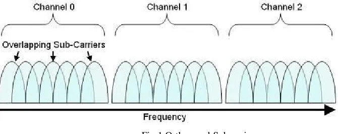
In OFDM is a subset of frequency division multiplexing in which a single channel utilizes multiple sub-carriers on adjacent frequencies. In addition the sub-carriers in an OFDM system are overlapping to maximize spectral efficiency. Ordinarily, overlapping adjacent channels can interfere with one another. However, sub-carriers in an OFDM system are precisely orthogonal to one another. Thus, they are able to overlap without interfering. As a result, OFDM systems are able to maximize spectral efficiency without causing adjacent channel interference. [6,7,8]
Fig 1.Orthogonal Subcarriers
Orthogonal frequency division multiplexing is commonly implemented in many emerging communications protocols because it provides several advantages over the traditional FDM approach to communications channels. More specifically, OFDM systems allow for greater spectral efficiency reduced inter-symbol interference (ISI), and resilience to multi-path distortion.
In mono-carrier systems, inter-symbol interference is often caused through the multi-path characteristics of a wireless communications channel. Note that when transmitting an electromagnetic wave over a long distance, the signal passes through a variety of physical mediums. As a result, the actual received signal contains the direct path signal overlaid with signal reflections of smaller amplitudes. In wireless systems, this creates difficulty because the received signal can be slightly distorted. In this scenario, the direct path signal arrives as expected, but slightly attenuated reflections arrive later in time. [9,10]
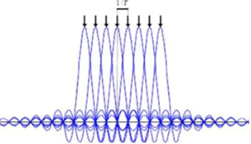
Fig.2. Basic Structure of Multicarrier System
In OFDM, the sub carrier pulse used for transmission is chosen to be rectangular. This has the advantage that the task of pulse forming and modulation can be performed by a simple Discrete Fourier Transform (DFT) which results in a remarkable reduction in equipment complexity (filters, modulators, etc.). In these references it is also shown that a multi tone data signal is effectively the Fourier transform of the original data stream, and that a bank of coherent demodulators at the receiver is effectively an inverse Fourier transform. However, since definitions have been changes afterwards, it is now said, that a multitone data signal is effectively the inverse Fourier transform of the original data stream and that a bank of demodulators is effectively a Fourier transform. Note that the (Inverse) Discrete Fourier Transform (IDFT) can be implemented very efficiently as an (Inverse) Fast Fourier Transform (IFFT). [14]
Consider the system shown in Figure 2.1. The input consists of a data symbol sequence dn that can be represented as an + jbn (where an and bn are real sequences representing the in-phase and quadrature components, respectively)
and, using the Inverse Fourier Transform, the transmitted waveform can be represented as:
However, for digital systems it is useful to consider the discrete case. In this case an Inverse Discrete Fourier Transform (IDFT) is performed at the transmitter on a vector.
d= (d0, d1, …,dN–1), the result is a vector D = (D0, D1, …, DN–1) with:
Where,
And s Mt =1/ fs (where fs is the symbol rate). Substituting t =NmMt in (2.1) and using (2.3) shows that the sampled sequence D (mMt) is in fact the IDFT of the sequence dn as shown in (2.2). Note that usually the whole
OFDM symbol is up converted to a specific carrier frequency of the RF band. If we again look to the OFDM symbol time it can be noticed that the signaling interval T has been increased to NMt, which makes the system less susceptible to delay spread impairments. Note that the act of truncating the rectangular signal to the interval (0, NMt ) in the time domain imposes a sin(x) / x frequency response on each sub channel with zeros at multiples of 1/T, which is the orthogonally principle of OFDM. [15, 16, 17]
At the receiver, the transmitted signals are recovered using the Discrete Fourier Transform. However, due to multipath distortion, the recovering of the transmitted signals brings some problems along.
way to increase system capacity is by transmitting data parallel on different frequencies. In classical parallel data systems, the total signal frequency band is divided into N non-overlapping frequency sub channels. In such systems, there is sufficient guard space between adjacent sub channels to isolate them at the receiver with N demodulators, i.e., one per sub channel. This solution, however, is very bandwidth inefficient. A more efficient use of bandwidth can be obtained with a parallel system if the spectra of the individual sub channels are permitted to overlap, with specific orthogonally constraints imposed to facilitate separation of the sub channels at the receiver.n the basis of such considerations, the algorithm uses a different color image multiplied by the weighting coefficients of different ways to solve the visual distortion, and by embedding the watermark, wavelet coefficients of many ways, enhance the robustness of the watermark.
III. IMPLEMENTATION
Consider a MIMO OFDM system with Nt transmit (TX) and Nr receive (RX) antennas. In addition to the spatial and temporal dimension of MIMO, OFDM adds one extra dimension to exploit, namely, the frequency dimension. In general, the incoming bit stream is first encoded by a one-dimensional encoder after which the encoded bits are mapped onto the three available dimensions by the Space-Time-Frequency (STF) mapper. After the STF mapper, each TX branch consists of almost an entire OFDM transmitter.
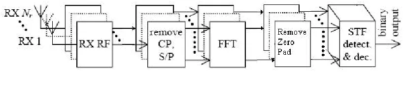
Fig 4 MIMO OFDM System
At receiver side, the CP is removed and the FFT is done per receiver branch. In the context of the unified view, at this point, overall STF detection and decoding must be performed to recover the binary data stream. In general, however, because the MIMO algorithms are single carrier algorithms, MIMO detection is performed per OFDM subcarrier. To that end, the received signals of subcarrier i are routed to the i-th MIMO detector to recover the Nt QAM symbols transmitted on that subcarrier. Next, the symbols per TX stream are combined.
Finally, STF de-mapping and decoding are performed on these Nt parallel streams and the resulting data are combined to obtain the binary output data.
Fig 5 STF De-mapping and decoding
Finally, note that OFDM has as advantage that it introduces a certain amount of parallelism by means of its Nc subcarriers. This fact can be exploited by MIMO OFDM.
Bussgang Algorithm
The operation of the blind channel equalizer is illustrated in Figure 5.1. Suppose we are given a signal u(n) which is the output from an LTI channel. The equalizer output is:
)
(
)
(
*
)
(
)
(
n
w
n
u
n
w
u
n
i
y
i
i
We then apply the filter output y(n) to a memory less nonlinear estimator g(y(n)) that acts as the desired response to an adaptive algorithm, such as the LMS algorithm. Clearly, we cannot use the channel input x(n) as our desired signal since it is unknown, so instead we must use some estimate of x(n) based upon observation of y(n). After computing the error e(n) = g(y(n)) − y(n), we update the tap weights. This general procedure is known as the Bussgang algorithm. Steps of Bussgang algorithm are:
1. Filtering: y(n) = wH(n) u(n) 2. Error computation: e(n) = g(y(n)) − y(n)
3. Updating: w(n + 1) = w(n) + µ u(n) e*(n)
In the LMS algorithm, the cost function J(n) = E[|e(n)|2] is a convex quadratic function of the tap weights and therefore has a unique minimum point. However, the cost function in the Bussgang algorithm is generally not a quadratic function due to the nonlinearity in g(y(n)). Therefore, the iterative de-convolution procedure may have several local minima in addition to global minima. For this reason, it is essential that the tap weight vector w(n) is initialized properly in order for w(n) to converge to the desired equalization filter.
For this algorithm to converge, we require the following mean-value convergence condition:
E[y(n)y(n − k)] = E[y(n)g(y(n − k))]
Any stochastic process y(n) that satisfies this condition is known as a Bussgang process. Clearly, we find that the validity of the algorithm depends on the proper nonlinear estimator g(·). For example, in a simple binary PAM
system where x(n) Є {−1, +1}, we can use the following estimator:
g(y(n)) = αsgn(y(n))
where the constant α is a data-dependent gain, given as:
]
)
(
[
)
(
2 2n
x
E
n
x
E
This choice of estimator results in a special case of the Bussgang algorithm, known as the Sato algorithm.
Constant-Modulus Algorithm
In the Sato algorithm, it can easily be seen that the gradient of the cost function reaches zero when perfect equalization is attained. However, if we use the same cost function for some M-array system such as M-array QAM or M-array PSK,convergencemay not be achieved. Instead, we can use a cost function that is suited for multi-dimensional communication systems, such as the following:
]
)
)
(
[(
)
(
p 2p
R
n
y
E
n
J
Where, the constant Rp ensures convergence of the algorithm:
And the error term is defined as follows:
)
)
(
(
)
(
)
(
)
(
n
y
n
y
n
p 2R
py
n
pe
The Bussgang algorithm that uses this choice of cost function is known as the Godard algorithm.
The Godard algorithm is more robust to phase perturbations than other Bussgang algorithms because it only relies on the magnitude of the received signal. The Sato algorithm is a special case of the Godard algorithm where p = 1. In the case of p = 2, we have the following values:
]
)
)
(
[(
)
(
2 22
R
n
y
E
n
J
]
)
(
[
]
)
(
[
2 4 2n
x
E
n
x
E
R
)
)
(
)(
(
)
(
n
y
n
R
2y
n
2e
The algorithm that uses this cost function is known as the constant-modulus algorithm (CMA). Steps of the CMA algorithm are: 1.Initialization
otherwise
M
i
w
i0
2
/
1
)
0
(
2. Filtering: y(n) = wH(n) u(n)
3. Estimation: g(y(n)) = y(n)(1 + R2 − |y(n)|2) 4. Error computation: e(n) = g(y(n)) − y(n)
5. Updating:w(n + 1) = w(n) + µ u(n) e*(n)
As stated before, the initial equalization is very important for the convergence of the Bussgang algorithm. So, we initialize the tap weight to 1 and all others to zero.
Linear Pre-coding
It belongs to the statistical class. It consists of a simple linear transformation applied to blocks of symbols before they enter the OFDM system, which enables blind channel estimation at the output of the OFDM system via cross-correlation operations. It does not introduce redundancy to the block, nor does it change the block length. The method is computationally simpler than deterministic methods, and its performance is comparable to that of sub space approaches at significantly lower complexity.
Let us consider an N-block OFDM system, and apply at its input a linear pre-coding block that performs the following task. It transforms the i-th OFDM block of N information symbols, [dik, k = 0,1……N-1] according to:
1
,....,
1
,
0
),
)
1
(
(
1
1
, , 2 ,
d
Ad
k
N
A
s
iTk k
i k
i
Where, T and A are both predefined numbers, assumed to be known to the transmitter and receiver; T is an integer in [0, N-1], and A is a pure imaginary number with |A| <1. This pre-coding has several properties:
It introduces no redundancy to the transmitted data, which makes the approach bandwidth efficient.
It preserves the transmission power on each subcarrier. We should note here that the requirement for A to be pure imaginary is necessary in order to maintain the power of the T-th carrier.
It maintains the zero-mean of the signal transmitted on each subcarrier.
It maintains zero DC offset in each block.
The coded block [si,k, k = 0,1…..N-1] goes through the regular OFDM transmission steps. The i-th received OFDM
block after removal of the CP and DFT is
1
,...,
0
)
1
(
)(
(
1
1
)
,
(
, . , , 2 , , ,
H
k
d
Ad
v
k
N
A
v
s
k
H
y
k iT ikk i k i k i k i
Where, H(k) is the complex gain of the k-th subcarrier, and vi,k models the noise. It is assumes that:
(i) The baud-rate channel can be modeled as an FIR filter of length L with tap coefficients h(l) , l = 0,1…..L-1, and hence,
1 0 2;
1
,...,
1
,
0
,
)
(
)
(
L l kl N jN
k
e
l
h
k
H
(ii)The channel stays the same for at least the duration of the block, and is quasi-stationary between blocks;
(iii)The noise vi,k is complex, circular Gaussian, zero-mean, white across subcarriers and blocks, and independent of
the information symbols.
The channel frequency response H(k), k = 0,1….N-1, or equivalently, the channel impulse response h(l), l = 0,1…..L-1, is needed in order to recover the transmitted signal si;k and consequently the information symbols di;k, k =
0,1…..N-1.
]
[
, *,,T i k i T
k
E
y
y
z
Based on zk,T, an estimate of the channel H(k) can be obtained as:
T
k
z
T
k
N
k
z
A
A
A
k
H
T k T k T k k,
,
1
,..
0
,
)
1
(
)
1
(
1
)
(
ˆ
, , 2 2The channel estimate can be further improved, (if the length of the channel is known) noting that Ĥ (k), k = 0,1….N -1, should be the DFT of the channel impulse response h(l), l = 0,1…..L--1, where L < N. The latter length constraint can be enforced by performing IDFT on ˆH (k), setting to zero the last N - L samples of the IDFT output, and then performing an N-point DFT on the result. This procedure is referred to as de-noising. A potential problem with the estimate might arise when the T-th carrier is in deep fade, in which case zk;T is close to zero for all k’s. However, it
is interesting to note that, at the receiver, any subcarrier can play the same role as the T-th one. Let R be an integer in [0,1….N-1] with R ≠ T. The channel response H(k) can be estimated as:
T
k
z
A
A
A
R
k
z
T
R
k
z
A
A
k
H
R k R T R R k R k R k , 2 * 2 , , 2 2)
1
(
)
1
(
1
,
,
,
)
1
(
1
)
(
ˆ
A criterion for selecting R can still be implemented at the receiver. It can be selected as:
1 0 2 ,max
arg
N k R k R oz
R
This step would require the estimation of the entire correlation matrix of the received blocks, thus introducing a small increase in complexity.
Scalar ambiguity
di;T is that, it varies from block to block, thus maintaining a zero-mean for the symbol transmitted over each carrier.
Thus, if di;T were to be set to some known value, this value would have to be assigned for each i by a pseudo-random
number generator. Perfect cooperation between transmitter and receiver would be needed in this case for the synchronization of the pilot sequence. The pilot could also be placed in the block after pre-coding. Assuming that one pilot is placed at location P in the pre-coded block, then, we can obtain an estimate of H(P) based on J received blocks as:
J i p i p is
y
J
p
H
1 , ,/
1
)
(
ˆ
wheresi;P is the pilot symbol used in block i. Subsequently, the channel estimate obtained before can be normalized
with respect to Ĥ (P).
Linear block pre-coding (LBP) has been used extensively for increasing throughput and diversity gains in MIMO OFDM systems. The design of codes to achieve these goals has recently become an area of huge interest and vast potential. For instance, algebraic number theory, coding theory, and iterative greedy optimization have being used to design optimal codes. However, very little work has been done on developing LBP schemes that allow channel estimation.
Consider a MR × MT , (MR≥MT ) MIMO OFDM system with ‘MT’ users and ‘MR’ receivers. A non redundant
linear block pre-coding is applied at the inputs before they enter the OFDM system, which increases multipath diversity and allows for blind channel estimation at the receiver. The channel estimation approach employs computationally simple cross-correlation operations and yields the channel up to a diagonal ambiguity. It does not require channel length information, and is not sensitive to additive stationary noise. The pre-coding does not increase transmission power and maintains even distribution of power between OFDM blocks. In a MR ×MT multi-user OFDM system the received symbol at the m-th receive antenna consists of contributions from all MT multi-users, given by:
1
,..
1
,
0
,
1
,...
1
,
0
),
(
)
(
)
(
)
(
1 0
R m i p M p mp im
k
H
k
s
k
n
k
k
N
m
M
y
T
where ‘i’ is the block index, ‘k’ is the carrier index ‘p’ is the user index, ‘sp(k)’ is the transmitted symbol over the k-th carrier, which, is derived from k-the source symbols dp(k) for k = 0, ...,N − 1; Hmp(k) is the gain of the k-th carrier between the m-th receive antenna and the p-th user; nm(k) denotes noise. ‘N’ is the block size.
Let di,P=[di,P(0)…di,P(N −1)]T denote the i-th block of symbols corresponding to the p-th user before any pre-coding.
During the i-th block, the symbols of the p-th user to be transmitted over carrier k are generated based on an N×1 code vector, wp(k; i), as:
si,p(k) = wHp (k; i) di.p
Equivalently, the i-th block of the p-th user is pre-coded according to:
si,p = [sip(0) ... sip(N − 1)]T = [ wp(0; i) , wp(1; i), ....,wp(N − 1; i) ]Hdi,P = Wi,pdi,p
whereWi,p is a matrix whose k-th row equals wHp (k; i).
The purpose of the pre-coding matrix is to introduce some correlation structure in the transmitted blocks. Also, by changing the coding matrix between subsequent blocks we will create diversity that will allow us to estimate the channel matrix. Since we will need to obtain autocorrelation estimates, the coding matrices have to stay the same for a number of blocks. Thus, take them to be periodic in i with period M, M ≥MT i.e.,
Wi,P = Wi+M,P
For the i-the received block, the symbols of all users that were received on carrier k in vector yi(k). It holds:
yi(k) = [yi, 0(k) ... yi,MR−1(k)]T = H(k) si(k) + n(k)
Where, si(k) = [si,0(k) .... si,MT−1(k)]T .
Where,
Consider a sequence of received symbols that start at block i and are spaced apart by M blocks:
)....}
(
),
(
),
(
{
)
(
k
y
k
y
k
y
2k
y
i
i iM i MThe correlation matrix of ˜yi(k), is given by:
1
,...
1
,
0
},
)
(
)
(
{
E
y
k
y
l
i
M
R
kli i i HIf Ukl is a full row rank matrix,
(
;
0
)
(
;
0
)
.
.
.
(
;
1
)
(
;
1
)
.
.
.
.
.
.
.
.
.
.
.
.
.
.
.
)
1
;
(
)
1
;
(
.
.
.
)
0
;
(
)
0
;
(
1 1 0 0 0 01
k
w
l
w
k
M
w
l
M
w
M
l
w
M
k
w
l
w
k
w
U
T T T M H M M H M H H kl AndThen to find the estimate,
kl ukl
lu
k
C
U
H
ˆ
(
)
III.EXPERIMENT AND RESULT
The following simulation results are displayed:
• Pilot Estimation (LS,MMSE)
• Blind Estimation (CMA, Pre-coding)
PILOT BASED ESTIMATION
Fig 6.1 SNR v/s MSE LS SISO plot
Fig 6.2 SNR v/s MSE MMSE MIMO plot
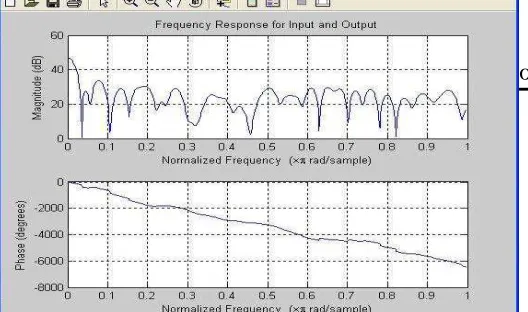
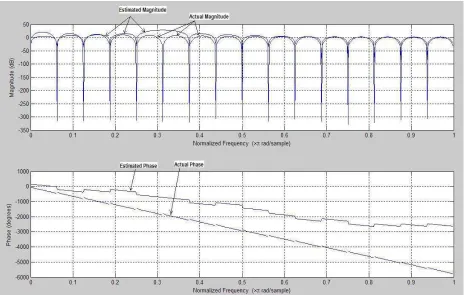
Fig 6.3 Frequency response of LS SISO
Fig 6.4 Frequency response of LS MIMO
Explanation: Here both the magnitude and phase response plots are plotted after the Normalization of Frequencies to 0 to 1 for SISO and MIMO systems using least squares method and from that figure it is clear that there are more fluctuations in SISO magnitude plot than MIMO, since SISO system is not stable as MIMO.
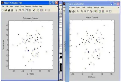
Fig 6.6 Actual and estimated channel scatter plots LS MIMO
Explanation: Here the scattered plot of inphase response of a channel for both SISO and MIMO systems are plotted.
Fig 6.8 MMSE MIMO channel scatter plots
Explanation :From the figure it is understand that the plots of channel scatters for SISO and MIMO systems are plotted.In both the plots almost Estimated plot is similar to the Actual Plot. Here every dot deals with the Inphase Response of the Channel.
BLIND ESTIMATION
Constant Modulus Algorithm
Explanation: It is the algorithm used for Indoor Environment. It is clearly seenthe MIMO is stable. Here the
estimated magnitude is compared with ideal output magnitude. In MIMO system the frequency response is improved than the SISO
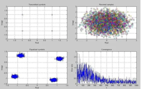
Fig 6.11 CMA Equalization
Explanation: Here we are equalizing the signals from the receiver with the help of transmitted signal statistics using CMA equalization and the result is approximately in equal to the Ideal value. In the convergence plot the error is reduced as the number of samples increases.
IV.CONCLUSION
Various channel estimation techniques are employed in order to judge the physical effects of the medium present. In this project, we analyze and implement various estimation techniques for MIMO OFDM Systems such as Least Squares (LS), Minimum Mean Square Error (MMSE), Constant Modulus Algorithm (CMA) and linear Pre-coding. These techniques are therefore compared to effectively estimate the channel in MIMO OFDM Systems.
REFERENCES
[1] B. Corona, Coleri, S., Ergen, M., Puri, A., and Bahai, A., “Channel Estimation Techniques Based on Pilot Arrangement in OFDM Systems,” IEEE Transactions on Broadcasting, vol. 48, pp. 223–229, Sept. 2002.
[2] Yang, B., Letaief, K. B., Cheng, R. S., and Cao, Z., “Channel Estimation for OFDM Transmission in Multipath Fading channels Based on Parametric Channel Modeling,” IEEE Transactions on Communications, vol. 49, pp. 467–479, March 2001.
[3] Sanzi, F., Sven, J., and Speidel, J., “A Comparative Study of Iterative Channel Estimators for Mobile OFDM Systems,” IEEE Transactions on Wireless Communications, vol.2, pp. 849–859, Sept. 2003.
[4] Li, Y., “Simplified Channel Estimation for OFDM Systems with Multiple Transmit Antennas,” IEEE Transactions on Communications, vol. 1, pp. 67-75, January 2002.
[6] S. Haykin, Ed., Blind Deconvolution. PTR Prentice Hall, Inc., 1994.
[7] Z. Ding and Y. G. Li, Blind Equalization and Identification, ser. Signal Processing and Communication Series. Marcel Dekker, Inc., 2001.
[8] H. Bolcskei, R.W. Heath, and A.J. Paulraj, “Blind channel identification and equalization in OFDM based multiantenna systems,” IEEE Trans. on Signal Processing, vol. 50(1), pp. 96-109, Jan. 2002.
[9] C.Y. Wong, R.S. Cheng, K.B. Letaief, and R.S. Murch, “Multiuser OFDM with adaptive subcarrier, bit, and power allocation,” IEEE Journal on Sel. Areas in Commun., vol. 17, no. 10, pp. 1747-1758, Oct. 1999.
[10] A. P. Petropulu, R. Zhang and R. Lin, “Blind OFDM Channel Estimation through Simple Linear Precoding,” IEEE Trans. on Wireless Communications, vol. 3, no. 2, pp. 647-655, Mar. 2004.
[11] S. Yatawatta and AthinaPetropulu, “Blind channel estimation in multiuser OFDM systems,” in Proc. 36th Asilomar Conf. on Signals Systems and Computers, vol. 2, pp. 1709-1713, Nov. 2002.
[12] M. Debbah, W. Hachem, P. Loubaton, and M. de Courville, “MMSE analysis of certain large isometric random precoded systems,” IEEE Trans. Inform. Theory, vol. 49, no. 5, pp. 1293 - 1311, May 2003.
[13] S. M. Alamouti, “A simple transmit diversity scheme for wireless communications,”IEEE J. Select. Areas Commun., vol. 16, pp. 1451–1458, Oct. 1998.
[14] A. Paulraj and C. B. Papadias, “Space–time processing for wireless communications,” IEEE Signal Processing Mag., vol. 14, pp. 49–83, Nov. 1997.
[15] H. Ge, K. D. Wong, and J. C. Liberti, “Characterization of multiple-input multiple-output (MIMO) channel capacity,” in Proc. IEEE Wireless Communications and Networking Conf. (WCNC), Orlando, FL, 2002.
[16] Y. Lin and S. Phoong, “BER minimized OFDM systems with channel independent precoders,” IEEE Trans. on Signal Processing, vol. 51, no. 9, pp. 2369-2380, Sep. 2003.