Super Mean Labeling and Square Difference Labeling of Some Graphs

Super Mean Labeling and Square Difference Labeling of Some Graphs

J. Ravi

_{S. Dickson}

_{H. Sabareesh}

_{J. Mohan}

_{G. Sathish Kumar}

1,2,3,4,5

_{Assistant Professor}

1,2,3,4,5

_{Department of Mathematics and Statistics}

1,2,3,4,5

_{Vivekanandha College For Women, Tiruchengode, Namakkal, Tamilnadu, India}

square difference labeling of some graphs. Let G be a (p,q) graph and f:v(G)→{1,2,3…p+q} be an injection for each edge e=uv ,let f*(e)=((f(u)+f(v)))/2 if f(u)+f(v) is even and f*(e)=(f(u)+f(v)+1)/2 if f(u)+f(v) is odd then f is called a super mean labeling if f(v)∪{f*(e):eϵE(G)}={1,2,3….P+q}. A graph that admits a super mean labeling is called a super

mean graph. The prove that

s(pn,k1),s(p2*p4),s(Bn,n),<Bn,n;pm>,Cn.k2,n≥3.Generalizd ant prism {An} and the double triangular snake D(Tn) are super mean graph. We proved that some new graphs admit square difference labeling. A function f is called a square difference labeling if there exists a bijection f: V(G)→{0,1,2,….p-1} such that the induced Function f*:E(G) → N given by f*(u v) = |[f(u)]2 - [f(v)]2| for every uv∈E(G) are all distinct. any graph which satisfies the square difference labeling is called a square difference graph .it is investigated that the central graphs of path, square graphs of path some path related graphs fan and gear graphs are all square difference graph.

Key words: Super Mean Labeling, Square Difference Labeling, Graph and Bijection

I. INTRODUCTION

Graph theory is an important branch of mathematics with relevance and application to the entire field. There are several reasons for the acceleration of interest in graph theory. The fact is that graph servers as a mathematical model for any system involving binary relation. Because of their diagrammatic representation, graphs have an intuitive and aesthetic appeal. Labeling of a graph is an assignment of labels to its vertices (or) and edges (or) faces, which satisfy some condition. In thirteenth century, Chinese mathematician Yang Hui and Oyhers (1275) have studied labeling of geometric figures which are later called plane graphs. Later Change Choo (1670), PaoChhi – Shou (1880), Li Nien also contributed to this area. Most graph labeling methods trace their origin to one introduced by Rosa (875) in 1967 or one given by Graham and Sloane (445) in 1980. Labeling graphs serves as useful modes for a broad range of applications such as coding theory, Radar astronomy, circuit designs and communication network. All graphs in this dissertation are finite, simple and undirected. The symbols V (G), E (G) will denote the vertex set and edge set of the graph (G). The cardinality of the edge set is called the size of G, A Graph with p vertices and q edges is called a (p,q) graph.

II. PRELIMINARIES

A. Definition: 2.1

A graph 𝐺 = {𝑉, 𝐸} consists of a set of objects 𝑉 = {𝑣1, 𝑣2, … , 𝑣𝑛} called vertices and another set 𝐸 =

{ 𝑒1, 𝑒2, … . … 𝑒𝑛} whose elements are called edges such that each ek is identified with an unordered pair of

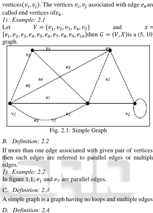
vertices(𝑣𝑖, 𝑣𝑗). The vertices 𝑣𝑖, 𝑣𝑗 associated with edge 𝑒𝑘are called end vertices of𝑒𝑘.

1) Example: 2.1

Let 𝑉 = {𝑣1, 𝑣2, 𝑣3, 𝑣4, 𝑣5} and 𝑥 =

{𝑒1, 𝑒2, 𝑒3, 𝑒4, 𝑒5, 𝑒6, 𝑒7, 𝑒8, 𝑒9, 𝑒10}then 𝐺 = (𝑉, 𝑋)is a (5, 10) graph.

Fig. 2.1: Simple Graph

B. Definition: 2.2

If more than one edge associated with given pair of vertices, then such edges are referred to parallel edges or multiple edges.

1) Example: 2.2

In figure 1.1, 𝑒1 and 𝑒7 are parallel edges.

C. Definition: 2.3

A simple graph is a graph having no loops and multiple edges.

D. Definition: 2.4

A walk of a graph 𝐺 is an alternating sequence of vertices and edges 𝑣0, 𝑥1, 𝑣1… . 𝑣𝑛−1, 𝑥𝑛, 𝑣𝑛 beginning and ending vertices such that each edge is incident with the vertices preceding and following it.

1) Example: 2.4

In figure 1.1, 𝑣1𝑒1𝑣2𝑒2𝑣3𝑒3𝑣4𝑒4𝑣1𝑒5𝑣3 is a walk.

E. Definition: 2.5

A walk which begins and ends at the same vertex is called a closed walk.

1) Example: 2.5

In figure 1.1, 𝑣1𝑒1𝑣2𝑒2𝑣3𝑒3𝑣4𝑒4𝑣1 is closed walk.

F. Definition: 2.6

The degree of a vertex 𝑣𝑖 of a graph, denoted by deg (𝑣𝑖), is the number of edges incident with that vertex.

1) Example: 2.6

In figure 1.1, degree(𝑣1) = 4.

G. Definition: 2.7

1) Example: 2.7

Fig. 2.2: Disconnected Graph

H. Definition: 2.8

A simple graph in which there exists an edge between every pair of vertices is called a complete graph or universal graph. The complete graph with p points is denoted by kp.

1) Definition: 2.9

A bi-graph (or) bipartite graph is one whose vertex set can be partitioned into 2 subsets v1and v2 such that each edge has one end in v1 and another end in v2.

Fig. 2.3: Bipartite Graph

I. Definition: 2.10

A graph is said to be labeled graph is its end vertices and its edges are distinguished from one another by some labels, such as letters (or) numbers.

Example: 2.10

Fig. 2.4: Labeled Graph

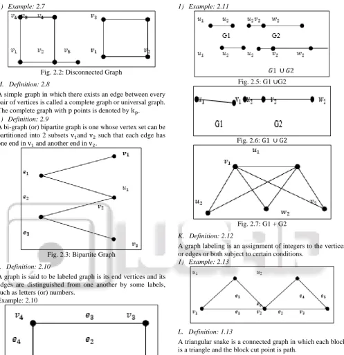
J. Definition: 2.11

Let G_1 = (v_1,x_1) and G_2= (v_2,x_2) be 2 graph with v_1⋃ v_2 =Φ.

We define, The union G_1⋃ G_2to be (V,X) where V=V_1

⋃ V_2and X= X_1⋃〖 X〗_2.

The sum G1+G2 as G_1 ⋃ G_2 together with all the edges joining vertices of v_1 to vertices of v_2.

1) Example: 2.11

Fig. 2.5: G1 ∪G2

Fig. 2.6: G1 ∪ G2

Fig. 2.7: G1 + G2

K. Definition: 2.12

A graph labeling is an assignment of integers to the vertices or edges or both subject to certain conditions.

1) Example: 2.13

L. Definition: 1.13

A triangular snake is a connected graph in which each block is a triangle and the block cut point is path.

III. SUPER MEAN LABELING OF SOME GRAPHS

A. Definition: 3.1

A function f is called a mean labeling of G if f:V (G) {0,1,2,3….,q} is injective and the induced function. f * : E(G) {1,2,……..q} defined as Let f*(e)= f(u)+ f(v)

2 if f (U) + f(v) is even f *(e) = f(u)+ f(v)+1

2 if f(U) + f ( v )is odd is bijective. The graph which admits mean labeling is called a mean graph.

B. Definition: 3.2

Let G be a (p, q) graph and f: V(G) {1, 2, 3,……., p + q

} be an injection. For each edge e=uv.Let f*(e)=f(u)+ f(v) 2 if f (U) + f(v) is even f *(e) = f(u)+ f(v)+1

Then f is called super mean labeling if f (V(G)) U { f*(e) : e€E (G)} = {1, 2, 3,………., p + q}. A graph that admits a super mean labeling is called super mean graph.

1) Example 3.1

Fig. 3.1: Super mean labeling. (P7: C6)

C. Definition: 3.3

Let u1, u2,……….,unui be the cycle Cm. Add vertices V1such that Vi is adjacent to ui, 1 ≤ i ≤ m. The resultant graph is Cm 1. Let w1, w2,………,wn be the path Pn. Let G = ( Cm 1) UPn whose edge set is E= { U1 Ui+1, UmU1 /1≤ i ≤ m -1 } U {w1 wi+1/1≤ i ≤ n-1} U. { Ui Vi / 1 ≤ i ≤ m – 1 }

1) Theorem: 3.1

Proof

V[

Fig. 3.2: ordinary labeling of (C3 K1) U Pn We label the vertices of (C3 K1) U Pn, f (u1) = 1; f (u2) = 3;

f (u3) = 5; f (u4) = 7; f (u5) = 10

f(u6) = 12; f (Vi) = 2i + 11, i = 1 to n Now the induced edge tables are as follows

f* (e1) = 2 ; f* (e2) = 4; f* (e3) = 6 ; f* (e4) = 9; f* (e5) = 11; f* (e6) = 8; f* (e1’ ) = 2i + 12, i = 1 to n and Clearly, f (v) U { f* (e): e € E(G)} = { 1, 2, 3, …….., p + q }.

So, f is a super mean labeling. Hence, (C3 K1) U Pn is a super mean graph for all n ≥ 2

1) Example: 2.3

Super mean labeling of (C3 K1) UP10 is give in figure 3.4

Fig. 3.3: Super Labeling of (C3 K1) UP10

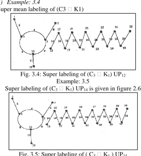
2) Example: 3.4

Super mean labeling of (C3 K1)

Fig. 3.4: Super labeling of (C3 1) UP12 Example: 3.5

Super labeling of (C3 1) UP14 is given in figure 2.6

Fig. 3.5: Super labeling of ( C3 1 ) UP14

D. Definition: 3.4

The graph ( Pn ; C3); the splitting graph is obtained by adding to each vertex v a new vertex V. So that V’ is a adjacent to every vertex is adjacent to V in ( Pn ; C3). The graph obtained by joining two copies of ( Pn ; C3) splitting graph.

1) Theorem: 3.2

( Pn ; C3) is a super mean graph for all n ≥ 2. Proof:

( Pn ; C3) is a graph with vertex set

V ( Pn ; C3) = { vi : 1 ≤ i ≤ n} U { vi'_{: 1 ≤ i ≤ n} U { ui : 1 ≤ i} ≤ n}U { u1'_{: 1 ≤ i ≤ n} and the edge set}

E (Pn; C3) = {ei: 1 ≤ i ≤ n - 1} U { ei'_{: 1 ≤ i ≤ n} U { e1}”_{: 1 ≤ i} ≤ n} U{ e1'”_{: 1 ≤ i ≤ n} U { e1}IV_{: 1 ≤ i ≤ n }}

The ordinary labeling of (Pn ; C3) is given in figure 2.7

Fig. 3.6: ordinary labeling of ( Pn ; C3) we label the vertices of ( Pn ; C3) as follows.

f (vi) = 9i – 1, i is odd, 1 ≤ i ≤ n – 1

9i – 8, i is even, 2 ≤ i ≤ n

f (vi’ ) = 9i – 3, i is odd, 1 ≤ i ≤ n – 1

9i – 6, i is even, 2 ≤ i ≤ n

f (ui) = 9i – 8, i is odd, 1 ≤ i ≤ n – 1

9i – 4, i is even, 2 ≤ i ≤ n

f (ui”) = 9i – 6, i is odd, 1 ≤ i ≤ n – 1

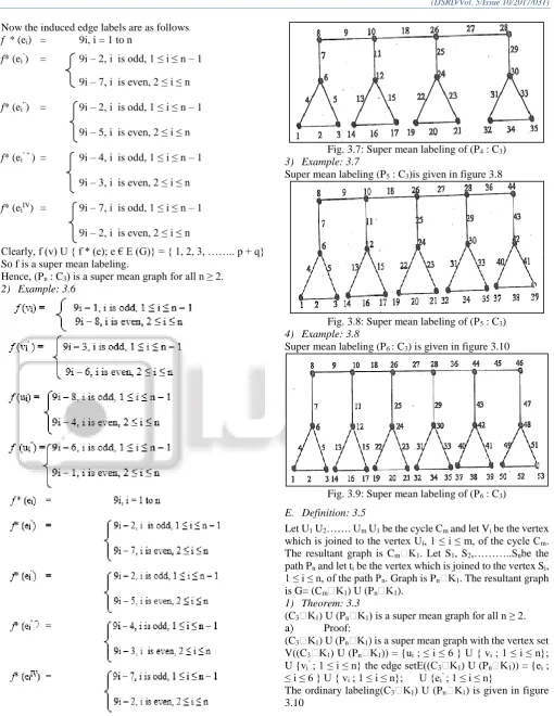
Now the induced edge labels are as follows f * (ei) = 9i, i = 1 to n

f* (ei’) = 9i – 2, i is odd, 1 ≤ i ≤ n – 1

9i – 7, i is even, 2 ≤ i ≤ n

f* (ei”) = 9i – 2, i is odd, 1 ≤ i ≤ n – 1

9i – 5, i is even, 2 ≤ i ≤ n

f* (ei’ “ ) = 9i – 4, i is odd, 1 ≤ i ≤ n – 1

9i – 3, i is even, 2 ≤ i ≤ n

f* (eiIV_{) = 9i – 7, i is odd, 1 ≤ i ≤ n – 1}

9i – 2, i is even, 2 ≤ i ≤ n

Clearly, f (v) U { f * (e); e € E (G)} = { 1, 2, 3, …….. p + q} So f is a super mean labeling.

Hence, (Pn : C3) is a super mean graph for all n ≥ 2. 2) Example: 3.6

Super mean labeling (P4 : C3) is given in figure 2.10.

Fig. 3.7: Super mean labeling of (P4 : C3) 3) Example: 3.7

Super mean labeling (P5 : C3)is given in figure 3.8

Fig. 3.8: Super mean labeling of (P5 : C3) 4) Example: 3.8

Super mean labeling (P6 : C3) is given in figure 3.10

Fig. 3.9: Super mean labeling of (P6 : C3)

E. Definition: 3.5

Let U1 U2……. Um U1 be the cycle Cm and let Vi be the vertex which is joined to the vertex Ui, 1 ≤ i ≤ m, of the cycle Cm. The resultant graph is Cm 1. Let S1, S2,………..Snbe the path Pn and let ti be the vertex which is joined to the vertex Si, 1 ≤ i ≤ n, of the path Pn. Graph is Pn 1. The resultant graph is G= (Cm 1) U (Pn 1).

1) Theorem: 3.3

(C3 1) U (Pn 1) is a super mean graph for all n ≥ 2. Proof:

(C3 1) U (Pn 1) is a super mean graph with the vertex set V((C3 1) U (Pn 1)) = {ui ; ≤ i ≤ 6 } U { vi ; 1 ≤ i ≤ n}; U {vi’ ; 1 ≤ i ≤ n} the edge setE((C3 1) U (Pn 1)) = {ei ; ≤ i ≤ 6 } U { vi ; 1 ≤ i ≤ n}; U {ei’ _{; 1 ≤ i ≤ n}}

Fig. 3.10: ordinary labeling of (C3 1) U (Pn 1) We label the vertices of ( C3 1 ) U (Pn 1)f (u1) = 1; f (u2) = 3; f (u3) = 5; f (u4) = 7; f (u5) = 10; f (u6) = 12;

Now the induced edge tables are as follows

f * (e1) = 2 ; f * (e2) = 4 ; f * (e3) = 6 ; f * (e4) = 9; f * (e5) = 11 ; f * (e6) = 8

f* _(e1’ _{) = 4i + 12, i = 1 to n ; f}* _(e1’’’ _{) = 4i + 10, i = 1 to n} Clearly, f (v) U { f* _{(e): e € E(G)} = { 1, 2, 3, …….., p + q }.} So, f is a super mean labeling. Hence ( C3 1 ) U (Pn 1) is a super mean graph for all n ≥ 2.

2) Example: 2.9

Super mean labeling of ( C3 1 ) U (Pn 1) is given in figure 3.12.

Fig. 3.11: super mean labeling ( C3 1 ) U (Pn 1) 3) Example: 2.10

Super mean labeling of (C3 1 ) U (Pn 1) is given in figure 3.13

Fig. 3.12: Super mean labeling of (C3 1 ) U (Pn 1)

REFERENCES

[1] Gallian. J.A, 2012, A dynamic Survey of graph labeling. The electronic Journal of Combinatories.

[2] Harary.F, 1988, Graph Theory, Narosa Publishing House Reading, New Delhi.

[3] Sandhya.S.S ,Somasundaram.S, Anusa.S, “Root Square Mean Labeling of Graphs” International Journal of Contemporary Mathematical Sciences ,Vol.9, 2014 , no.14 , 667-676.

[4] Sandhya.S.S ,Somasundaram.S, Anusa.S, “Some More Results on Root Square Mean Graphs” ,Journal of Mathematics Research , Vol.7,No.1;2015.

[5] Sandhya.S.S ,Somasundaram.S , Anusa.S, “Root Square Mean Labeling of Some New Disconnected Graphs” International Journal of Mathematics Trends and Technology, volume 15, number 2, 2014.page no:85-92. [6] Sandhya.S.S ,Somasundaram.S , Anusa.S, “Root Square

Mean Labeling of Subdivision of Some More Graphs” International Journal of Mathematics Research, Volume 6, Number 3, 253-266.

[7] Sandhya.S.S ,Somasundaram.S , Anusa.S, “Some New Results on Root Square Mean Labeling” International Journal of Mathematical Archive -5(12), 2014, 130-135. [8] Sandhya.S.S , Somasundaram.S , Anusa.S, Root Square

Mean Labeling of Subdivision of Some Graphs” Global Journal of Theoretical and Applied Mathematics Sciences, Volume 5, Number 1, (2015) pp.1-11. [9] Sandhya.S.S ,Somasundaram.S , Anusa.S, “Root Square

Mean Labeling of Some More Disconnected Graphs”, International Mathematical Forum, Vol.10, 2015, no.1 , 25-34.