A NOVEL APPROACH FOR SEGMENTING COMPUTER
TOMOGRAPHY LUNG IMAGES USING ECHO STATE
NEURAL NETWORKS
1DR.Z. FAIZAL KHAN, 2DR. S. VEERAMALAI, 3DR.G.NALINI PRIYA, 4M.RAMESH KUMAR,
5A. NARESH KUMAR. 6DR A. KANNAN.
1Associate professor, Dept of CSE, IAJJCE, Nagercoil, Tamilnadu, India
2Professor, Vel Tech High Tech Dr. Rangarajan Dr. Sakunthala Engineering College, India.
3
Professor, Det of IT, Saveetha Engineering College, Chennai, India.
4.5Assistant Professor, Dept of CSE, Agni College of Technology, Chennai, India.
6Professor and Head, Dept of Information Science and Technology, Anna University Chennai, India,
ABSTRACT
Segmentation is an important step for finding out the different portions of an image. Existing segmentation algorithms have involved many stages like elimination of blood vessels, tissues and finally showing the nodule in the segmented image. This paper proposes new segmentation technique using recurrent Echo State Neural Network (ESNN) method on computer tomography (CT) lung image. ESNN has been chosen in this work since it reduces the number of steps in segmentation to identify the presence of nodules in the CT lung image. The performance of ESNN segmentation has been shown to be the best when compared with other conventional segmentation algorithms like ‘Sobel’, ‘Prewitt’, ‘Robertz’, ‘Log’, ‘Zerocross’, ‘Canny’ and Contextual clustering. Matlab regionprops function has been used as one of the criteria to show the performance of segmentation algorithms. From this research work, it has been observed that the segmentation accuracy of the proposed algorithm has been achieved to 84.40%.
Keywords: Echo State Neural Network, Contextual Clustering, Segmentation Performance, CT Lung
Image.
1. INTRODUCTION
Image segmentation is an important task
for image understanding and analysis.
Segmentation partitions an image into a set of
different regions based on its intensity
properties, so that each region is homogeneous with respect to certain intensity characteristics. The various regions segmented in an image can be further used for different types of interpretations. Segmentation of image involves extracting features and deriving metrics to segregate regions of homogeneous intensities. This can be achieved by choosing a selective region of interest or by considering the entire image. Many image segmentation methods have been proposed earlier for the process of successive image analysis. Existing methods have used mostly thresholding concepts for
segmenting various regions of interest. In addition, the following methods have been used
for segmentation: statistical methods,
geometrical methods, structural methods, model based methods, signal processing methods, spatial domain filters, Fourier domain filtering, Gabor and wavelet models.
Lung nodules indicate lung
abnormalities in a human lung. A pulmonary nodule is the most common manifestation of lung cancer. Lung nodules are approximately-spherical regions of relatively high density that are visible in X-ray images of the lung. Large (>1 cm in diameter) malignant nodules can be detected with traditional imaging equipment and can be diagnosed by needle biopsy or
bronchoscopy techniques. However, the
are limited due to problems associated with accessing small tumors, if they are located inside the tissue. Hence, additional diagnostic and imaging techniques are needed. One of the most promising techniques for detecting small cancerous nodules relies on characterizing the nodule based on its growth rate. The growth rate is estimated by measuring the volumetric change of the detected lung nodules over time. Hence, it is important to accurately measure the volume of the nodules to quantify their growth rate over time. Early detection of nodules can help in saving lung patients. Lung nodules can be detected by radiologists through examining lung images. Nodules and nodular patterns are seen both in chest radiographs and in CT scans. A single nodule has the appearance of a rounded or irregular opacity, which may be defined as follows: solid, non-solid or partly solid; and soft tissue or Ground-Glass Opacity (GGO) which is less than 3 cm diameter, Hansell et al. [6]. Therefore, automatic lung nodule detection (ALND) in the computer tomography (CT) images is still a challenging task. Inspite of lot of
mathematical algorithms that have been
developed over the period of years, still intervention and suggestions by a good radiologist is a must.
Chest Computer Tomography (CT) is a good approach for an effective pulmonary image analysis. The CT images have been used for the diagnosis of various pulmonary diseases such as
Lung cancer, Tuberculosis, Pulmonary
embolism. In this paper, we provide a new technique for segmenting CT lung image by adopting the Echo State Neural Network
(ESNN). The application of Contextual
clustering (CC) by Eero Salli [2, 20, 21] was proposed for functional magnetic resonance image (fMRI) analysis. In this paper, CC has also been used for segmenting the CT Lung image. Echo State Neural Network was proposed by Jaeger [8, 9] for learning system dynamics. We have proposed ESNN for effective segmentation of CT lung images. ESNN has not been used earlier for CT lung image segmentation.
The remainder of this paper is organized as follows: Section 2 provides a survey of related work in this area and compares them with the work proposed in this thesis. Section 3 explain the problem definition and provides new technique for segmenting lung CT images. Section 4 depicts the experimental results. Section 5 presents the conclusion on this work and suggests some possible future enhancements.
2. RELATED WORKS
There are many works in the literature that discuss about lung image analysis. From these works, it is observed that first hand assessment of lung affected patients for radiologic diagnosis is by using cross-sectional and projectional imaging techniques. Hansell [7] investigated structure-function relationships in lung disease with high-resolution CT image. The author claims that the CT imaging provides
better identification, localization, and
quantification of small lung nodules. Ted et al [15] studied the effect of computer-aided diagnosis (CAD) on radiologists' estimates of the likelihood of malignancy of lung nodules on computed tomography (CT) images. Wallace et al. [16] have discussed Ground-Glass Opacity (GGO). It is defined as increased attenuation of lung parenchyma without obscuration of the pulmonary vascular markings on CT images. It is considered one of the important features in lung cancer diagnosis of CAD.
Anti-geometric diffusion has been used as preprocessing to remove image noise. Geometric shape features (such as shape index and dot enhancement), are calculated for each voxel within the lung area to extract potential nodule concentrations. Rule based filtering is then applied to remove False Positive regions Ye et al. [18]. Golosio et al [5] used multislice computed tomography (MSCT) for lung cancer detection and identify noncalcified nodules of small size (from about 3 mm). The authors had used region of interest (ROI) based on a multithreshold surface-triangulation approach. Diagnosis of pulmonary infections using texture
classification was carried out by Yao et al. [17]. Application of CAD in medical imaging has been presented by Giger et al [4].
The existing methods for LND have used different stages of image processing according to the user requirements. Each intermediate stages of image processing have been discussed by Lee et al [10]. Automated
voxel-by-voxel classification of airways,
fissures, nodules, and vessels from chest CT images using a single feature set and classification method have been done by Ochs et al. [12]. Segmentation of lung high resolution CT (HRCT) images using a pixel-based approach has been used by Garnavi et al [3]. The
authors have used global-threshold
segmentation, mathematical morphology, edge detection, noise reduction, and geometrical computations to achieve the defined ROIs.
A Neural network-based fuzzy model has been proposed by Lin et al [11] to detect lung nodules. The authors used a set of appropriate fuzzy inference rules, and refine the membership functions through the steepest gradient descent-learning algorithm. A specific gray-level mathematical morphology operator acting in the 3D space of the thorax volume was defined by Catalin et al [1] in order to discriminate lung nodules from other dense (vascular) structures. The proposed method detects isolated, juxtavascular and peripheral nodules with sizes ranging from 2 to 20 mm diameter.
A multiscale joint segmentation and model fitting solution which extends the robust mean shift-based analysis to the linear scale-space theory was proposed by Okada et al. [13]. In their work, an ellipsoidal (anisotropic) geometrical structure of pulmonary nodules in the multislice X-ray computed tomography (CT) images have been used for target’s center location, ellipsoidal boundary approximation, volume, maximum/average diameters.
From the works found in the literature, it has been observed that most of the existing
works used ROC and thresholding for
segmentation. However, in case of medical applications, the accuracy provided by these
techniques is not sufficient to make effective decisions. Therefore, it is necessary to propose a new and efficient technique to enhance the accuracy of segmentation.
3. PROBLEM DEFINITION
The purpose and the contribution of this paper is to propose a new technique using Echo State Neural Network (ESNN) for proving
improved segmentation that guarantees
continuity inside each segmented object of the CT Lung image. This algorithm helps in identifying low contrast and high intensity nodules.
Feature extraction
In general, features can be defined as follows:
1. The range of intensity values in a 3 X 3
pixels or 5 X 5 or 7 X 7 or 9 X 9 pixel during segmentation process. Statistical calculations like mean, min, max, histogram etc can be applied on the block of pixels
2. The range of intensity values, fiducial
points on the edges of the predefined shapes can be features. The lung nodules do not have a definite shape. The nodules are irregular in shape with varying volumes. The intensity values that represent these nodules will vary in different CT slices
3. The ‘regionprops’ function in Matlab
2011a offers the following features for each objects in the segmented CT lung
image. The features are: 'Area',
'Perimeter', 'Solidity'. These features can be obtained from the segmented ‘bwlabel’ four connected pixels. Echo state neural network
has been found to possess a highly interconnected and recurrent topology of nonlinear PEs that constitutes a reservoir of rich dynamics and contains information about the history of input and output patterns. The outputs of this internal PEs (echo states) are fed to a memory less but adaptive readout network that produces the network output. The interesting property of ESNN is that only the memory less readout is trained, whereas the recurrent topology has fixed connection weights. This reduces the complexity of RNN training to simple linear regression while preserving a
recurrent topology, but obviously places
important constraints in the overall architecture that have not yet been fully studied.
The echo state condition is defined in terms of the spectral radius (the largest among the absolute values of the eigenvalues of a matrix, denoted by (|| ||) of the reservoir’s weight matrix (|| W || < 1). This condition states that the dynamics of the ESNN is uniquely controlled by
the input, and the effect of the initial states vanishes. The current design of ESNN parameters relies on the selection of spectral radius. There are many possible weight matrices with the same spectral radius, and unfortunately they do not perform at the same level of mean
square error (MSE) for functional
approximation.
The recurrent network is a reservoir of highly interconnected dynamical components, states of which are called echo states. The memory less linear readout is trained to produce the output. Consider the recurrent discrete-time neural network given in Figure 1 with M input units, N internal PEs, and L output units. The
value of the input unit at time n is u(n) = [u1(n),
u2(n), . . . , uM(n)]T ,
The internal units are x(n) = [x1(n), x2(n), . .
. , xN(n)]T , and
Output units are y(n) = [y1(n), y2(n), . . . , yL (n)]T.
Figure 1. Echo State Network
The connection weights are given
• in an (N x M) weight matrix
back ij
back
W
W
=
for connections betweenthe input and the internal PEs,
• in an N × N matrix ijin
in
W
W
=
forconnections between the internal PEs
• in an L × N matrix ijout
out
W
W
=
forconnections from PEs to the output units and
• In an N × L matrix ijback
back
W
W
=
for theconnections that project back from the output to the internal PEs.
The activation of the internal PEs (echo state) is updated according to
x(n + 1) = f(Win u(n + 1) + Wx(n) +Wbacky(n)),
Here, all fi’s are hyperbolic tangent
functions
x x
x x
e
e
e
e
− −
+
−
. The output from the readoutnetwork is computed according to y(n + 1) = fout(Woutx(n + 1)), .
Where
f
out=
(
f
1out,
f
2out,....,
f
Lout)
are theoutput unit’s nonlinear functions. Generally, the readout is linear so fout is identity [14].
Pattern generation for training ESNN
A total of 258064 blocks are obtained. In each block, average intensity is found and target value as 0.1(black) or 0.9(white) is allotted. The allotment of target value is based on the histogram plot (Figure 42). The x-axis represents the intensity values of the DICOM image. Y-axis represents the frequency of the intensity values. The average value obtained from each block along with the target allotted is treated as pattern. Hence, 258064 patterns are obtained. Patterns with similar values are removed by sorting and hence approximately less than 1000 patterns are obtained. The final number of patterns varies depending on the contents of the CT slice.
ESNN algorithm consists of two phases namely Training and Testing (segmentation) Phase 1: Training ESNN
Step 1: Read 31st slice in DICOM format and separate the image into 3 x 3 overlapping blocks of pixels.
Step 2: Decide the number of reservoirs.
Step 3: Decide the number of nodes in the input layer = 3.
Step 4: Decide the number of nodes in the output layer = number of target values=1.
Step 5: Initialize state vector (number of reservoirs)=0.
Step 6:Initialize random weights between input layer (IL) and hidden layer(hL). Initialize
weights between output layer(oL) and
hidden layer (hL). Initialize weights in
the reservoirs.
Step 7:Calculate state_vectornext = tanh
((ILhL)weights*Inputpattern +(hL)weights* state vectorpresent+(hLoL)weights * Targetpattern). Step 8:Calculate, a = Pseudo inverse (State vector all patterns).
Step 9:Calculate, Wout = a * T and store Wout for segmentation.
Phase II: Testing (Segmentation)
Step 1: Adopt step 1 and step 2 mentioned in Training.
Step 2: Calculate state_vector= tanh ((ILhL)weights*Inputpattern +(hL)weights* state vectorpresent+(hLoL)weights * Targetpattern). Step 3: Estimated output= state_vector * Wout Step 4: Assign 0 (black) or 255(white) in the
new matrix which will be the
[image:5.595.88.290.578.699.2]segmented image.
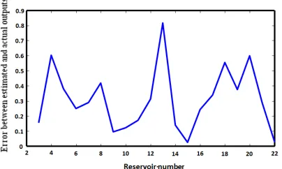
Figure 4. Error Between Estimated And Actual Output Figure 5.Error Between Estimated And Actual Output
Figure 2 shows the error between estimated and target values for different number of reservoirs. The number of reservoirs decides the recalling of the stored patterns. The optimal number of reservoirs is 22. The plot shows minimum error at reservoir numbers 3, 7, 15 and 22 which can be noticed in the x-axis. The curve
oscillates the minimum error and best
segmentation is obtained with 22 reservoirs. The effect of segmentation is influenced by the initial weight normalization between input layer and hidden reservoirs, inside hidden reservoirs, between reservoirs and output layer.
Figure 3 presents error between estimated and target values during normalization of weights between reservoir and inputs. Better segmentation is possible when the weight normalization is between 0.4 and 0.6 between input layer and the reservoirs.
Figure 4 presents impact of weight normalization inside reservoir for segmentation error through estimated output and target values. Better segmentation is possible when the weight normalization is between 0.2 and 0.3 inside reservoirs.
In Figure 5, the change of weight values and their impact in estimation by ESNN is presented when the weight normalization is done only between output layer and hidden layer (reservoirs). The error increases and decreases. The x-axis represents the change in the weight values in output and hidden layer. Better segmentation is possible when the weight normalization is between 2 and 3 between input layer and the reservoirs.
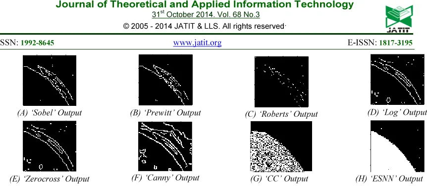
[image:6.595.196.401.551.713.2](A) ‘Sobel’ Output (B) ‘Prewitt’ Output (C) ‘Roberts’ Output (D) ‘Log’ Output
[image:7.595.91.522.72.260.2](E) ‘Zerocross’ Output (F) ‘Canny’ Output (G) ‘CC’ Output (H) ‘ESNN’ Output Figure 7. Segmentation Outputs For The Rectangular Block ‘A’ Shown In Figure 7
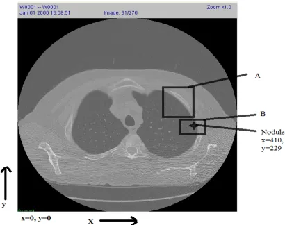
Figure 6 shows the 31st slice with rectangular
box ‘B’ showing the nodule location at x=410
and y=229. Figure 6 shows the 31st slice with
rectangular box ‘A’. As a comparison purpose, segmentation of a portion of image slice by different methods have been shown for the
[image:7.595.83.522.84.484.2]portion of Figure 6. Figures (7 a-g) show the segmentation by ‘Sobel’, ‘Prewitt’, ‘Roberts’, ‘Log’, ‘Zero crossing’, ‘Canny’ and ‘Contextual clustering’ methods. Matlab ‘bwlabel’ function has been used and the number objects for each method is shown in Figure 11.
Figure 8. Output Of ESNN For The Output Given In Figure 8h Figure 8 presents ESNN estimate with
values less than 210. This is based the small area considered for segmentation. The values in the y-axis do not correspond to the intensity values. The y-axis represents the estimates of ESNN.
The x-axis represents the number of overlapping windows used for segmentation. The threshold fixed for ESNN segmentation is based on the ranges of estimation.
(A) ‘Sobel’ Output (B) ‘Prewitt’ Output (C) ‘Roberts’ Output (D) ‘Log’ Output
[image:7.595.81.508.250.621.2](E) ‘Zerocross’ Output (F) ‘Canny’ Output (G) ‘CC’ Output (H) ‘ESNN’ Output Figure 9. Segmentation Outputs For The Block ‘B’ Shown In Figure 7
Figure 9 Shows segmentation outputs. The outputs by ‘Sobel’, ‘Prewitt’, ‘Roberts’, ‘Log’, ‘Zero crossing’, ‘Canny’ are almost blank
[image:7.595.86.501.406.682.2] [image:7.595.96.497.557.686.2](x=410, x=229) along with other information without noise. By using nodule template, the nodule can be located. The segmented output is through only one stage when compared to other methods that involved many stages (as per literature).
Performance comparisons
The cropping window shown in Figure 6 (block ‘A’) has few objects. The segmented
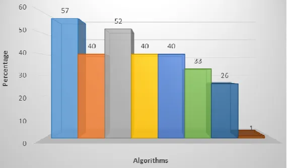
objects are thinned and can be noticed in Figures (7a-f). The segmented object in the Figure 7g shows more area and with tiny objects instead of one single object. Figure 8h has one solid object obtained from ESNN segmentation process. From Figure 10, it can be noticed that the ESNN has one object. Other segmentations methods show more number of objects.
Figure 10. Number Of Objects In Each Segmentation Method
The segmentation accuracy Asis
computed using the following equation used in [19] to evaluate the quality of the segmentation results:
gion SegmentedRe I
Objects of Number
) Perimeter' '
Area' ' Solidity' ('
S
+ +
= (1
)
gion d Unsegmente Perimeter Area
Solidity Re
I (' ' ' ' ' ')
O = + +
(2)
100
*
O
S
A
I I
s
=
(3)Where, SI denotes the number of correctly
segmented pixels, and OI represents the total
[image:8.595.156.442.256.423.2]number of pixels in the specified image. In this work, number of objects, ‘Solidity’, ‘Area’ and ‘Perimeter’ have been used as the criteria for finding the segmentation accuracy of the algorithms.
Table 1. Segmentation Accuracy Of Proposed Method
Algorithms No of objects ‘Area’ ‘Solidity’ ‘Perimeter’ Segmentation %
Sobel 57 43 0.253 96.5 5.0909
Prewitt 40 40 0.292 93.4 4.8727
Robertz 52 5 0.100 11.3 0.5964
Log 40 80 0.102 197.0 10.0727
Zerocross 40 80 0.102 197.0 10.0727
Canny 33 115 0.150 194.0 11.2364
CC 26 1490 0.250 198.0 82.1545
4. CONCLUSION
In this paper, a novel segmentation approach by applying feature selection and segmentation using Echo state neural network has been proposed. The main purpose of proposing ESNN based segmentation method is that it provides more accuracy in segmenting CT Lung images. The major advantage of this approach is the segmented objects don’t require additional morphological processing. It Increases the number of pixels to enhance the continuity of the segmented objects. The segmented results obtained from each segmentation algorithms are further processed using ‘bwlabel’ functions in order to indicate the number of objects presents in it. An ROI with one region has been cropped from the original image and used as inputs for each segmentation algorithm. ESSN results in more number of pixels through ‘Solidity’, ‘Area’ and ‘Perimeter’. Our proposed approach results in more ‘Solidity’, ‘Area’ and ‘Perimeter’
compared to Conventional segmentation
methods.
REFERENCES:
[1] Catalin I. Fetita, Françoise Prêteux,
Catherine Beigelman-Aubry and Philippe Grenier, 2003, 3-D automated lung nodule segmentation in HRCT- Lecture Notes in
Computer Science, Medical image
computing and computer-assisted
intervention-MICCAI, Vol. 2878/2003, pp. 626-634, DOI: 10.1007/978-3-540-39899-8_77.
[2] Eero Salli, Hannu J. Aronen, Sauli
Savolainen, Antti Korvenoja, and Ari Visa, 2001, Contextual Clustering for Analysis of Functional MRI Data, IEEE transactions on medical imaging, Vol. 20, No. 5, pp. 403-414.
[3] Garnavi R, Baraani-Dastjerdi A, Abrishami
Moghaddam H, 2005, A new segmentation method for lung HRCT images, Proceedings
of the Digital Imaging Computing:
Techniques and Applications, p.8. IEEE CS Press, Cairns Convention Centre, Brisbane, Australia, <doi>10.1109/DICTA.2005.5.
[4] Giger ML, Chan HP, Boone J, 2008,
Anniversary paper: history and status of CAD and quantitative image analysis: the role of medical physics and AAPM. Medical Physics, Vol. 35, Issue 12, pp. 5799–5820.
[5] Golosio B, Masala GL, Piccioli A, Oliva P,
Carpinelli M, Cataldo R, 2009, A novel multi-threshold method for nodule detection in lung CT. Medical Physics, Vol. 36, Issue 8, pp. 3607–3618.
[6] Hansell DM, Bankier AA, MacMahon H,
McLoud TC, Muller NL, Remy J, 2008, Fleischner society: glossary of terms tor thoracic imaging. Radiology, Vol. 246, Issue 3, pp. 697–722.
[7] Hansell DM. 2000, Imaging the lungs with
computed tomography, IEEE Engineering in Medicine and Biology Magazine, Vol. 19, Issue 5, pp. 71–79.
[8] Jaeger H., 2001, Short term memory in echo
state networks. Technical Report GMD Report 148, German National Research Center for Information Technology.
[9] Jaeger H., 2003, Adaptive nonlinear system
identification with echo state networks.
[10]Lee SLA, Kouzani AZ, Hu EJ, 2012,
Automated detection of lung nodules in computed tomography images: a review, Machine Vision and Applications, Vol. 23, Number 1, pp. 151-163.
[11]Lin DT, Yan CR, Chen WT, 2005,
Autonomous detection of pulmonary
nodules on CT images with a neural network-based fuzzy system, Comput. Med. Imaging Graph, Vol. 29, pp. 447–458.
[12]Ochs RA, Goldin JG, Abtin F, Kim HJ,
Brown K, Batra P, Roback D, McNitt-Gray
MF, Brown MS, 2007, Automated
classification of lung bronchovascular
anatomy in CT using Adaboost, Med. Image Anal. Vol. 11, pp. 315–324.
[13]Okada K, Comaniciu D, Krishnan, 2005, A
Robust Anisotropic Gaussian Fitting for Volumetric Characterization of Pulmonary Nodules in Multislice CT, IEEE Trans. Med. Imaging, Vol. 24, No. 3, pp. 409–423.
[14]Purushothaman S and Suganthi D, 2008,
network, International Journal of Image Processing, Vol. 2, Issue 1, pp.1-9.
[15]Ted Way, Heang-Ping Chan, Lubomir
Hadjiiski, Berkman Sahiner, Aamer
Chughtai, Thomas K. Song, Chad Poopat, Jadranka Stojanovska, Luba Frank, Anil Attili, Naama Bogot, Philip N. Cascade, Ella A. Kazerooni, 2010, Computer aided diagnosis of lung nodules on CT scans: ROC study of its effect on radiologists’ performance. Academic Radiology, Vol. 17, Issue 3, pp. 323–332.
[16]Wallace T, Millar Jr and Rosita M. Shah,
2005, Isolated diffuse Ground –Glass opacity in Thoracic CT, causes and clinical
presentations, American journal of
Roentgenology, Vol.184, pp. 2613-2622.
[17]Yao J, Dwyer A, Summers RM, Mollura DJ,
2011, Computer-aided diagnosis of
pulmonary infections using texture analysis and support vector machine classification, Academic Radiology, Vol. 18, Issue 3, pp. 306–314.
[18]Ye X, Lin X, Beddoe G, Dehmeshki J, 2007,
Efficient computer-aided detection of
ground-glass opacity nodules in thoracic CT images, Conf Proc IEEE Eng Med Biol Soc, pp. 4449–4452.
[19]Faizal Khan, Z & Kannan, “Intelligent
Segmentation of Medical images using
Fuzzy Bitplane Thresholding”,
“Measurement science and Review, Vol 14, No 2, pp-94-101, 2014.
[20]Faizal Khan, Z & Kavitha, V 2012,
‘Estimation of objects in Computed
Tomography Lung Images using
Supervised Contextual Clustering’,
Research Journal of Applied Sciences, vol. 7, no. 9-12, pp.494-499
[21]Faizal Khan, Z & Kavitha, V 2012,