R E S E A R C H
Open Access
Finite difference approach for variable
order reaction–subdiffusion equations
M. Adel
1**Correspondence: [email protected] 1Department of Mathematics, Faculty of Science, Cairo University, Giza, Egypt
Abstract
The fractional reaction–subdiffusion equation is one of the most famous subdiffusion equations. These equations are widely used in recent years to simulate many physical phenomena. In this paper, we consider a new version of such equations, namely the variable order linear and nonlinear reaction–subdiffusion equation. A numerical study is introduced using the weighted average methods for the variable order linear and nonlinear reaction–subdiffusion equations. A stability analysis of the proposed method is given by a recently proposed procedure similar to the standard John von Neumann stability analysis. The paper is ended with the results of numerical examples that support the theoretical analysis.
MSC: 65N12; 65M60; 41A30
Keywords: Weighted average finite difference approximations; Variable order linear and nonlinear reaction–subdiffusion equation; Stability analysis; Numerical example
1 Introduction
Fractional calculus is a very hot area of research due to its ability to study many appli-cations in physics and engineering, which cannot be studied by the ordinary calculus. There are many applications of this important type of calculus [1–4]. The approximate and numerical techniques must be used [5–9] because most fractional differential equa-tions (FDEs) do not have exact soluequa-tions. Recently, several numerical methods to solve fractional differential equations have been proposed, such as variational iteration method [10], homotopy perturbation method [11], Adomian decomposition method [12], homo-topy analysis method [13], finite difference method (FDM) [14,15], and spectral methods [5,6].
Many physical processes appear to exhibit fractional order behavior that may vary with time or space. This fact enables us to consider the order of the fractional integrals and derivatives to be a function of time or some other variables. The objective of this work is to identify the most appropriate definition of a variable-order operator for modeling dynamic systems and to assign the order of the derivative to give a physical meaning that will facilitate the understanding of its use in problems of vibration and control. However, until now, only few researchers have considered the numerical analysis of variable-order differential equations; see, for example, [16–20].
In this paper, we study the following variable order linear and nonlinear reaction–
where we assume Dirichlet boundary conditions as follows:
y(0,t) =φ(t), y(L,t) =ψ(t), 0 <t≤T, (2)
with an initial condition
y(x, 0) =ω(x), 0≤x≤L. (3)
On a finite domaina<x<b, 0≤t≤T, wheref is the source term, which may be linear (g(x,t)) or nonlinear (g(x,t,y(x,t))), 0 <γ(x,t) < 1,εis a positive constant and D1–t γ(x,t) is the variable order fractional derivative defined by the Riemann–Liouville operator of order 1 –γ, which is defined for a functionf(x,t) by (see [18,20])
And we use the weighted average FDM to solve this model.
2 Fractional reaction–subdiffusion equation
The standard mean-field model for the evolution of the concentrationsa(x,t) andb(x,t) of A and B particles is given by the reaction–diffusion equations:
∂
whereDis the diffusion coefficient assumed in this paper to be equal for species andεis the rate constant for the bimolecular reaction.
In order to generalize the reaction–diffusion problem to a reaction–subdiffusion prob-lem, we must deal with the subdiffusive motion of the particles. Seki et al. [21] and Yuste et al. [22] replaced Eqs. (5) and (6) with the set of reaction–subdiffusion equations, in which both the motion and the reaction terms are affected by the subdiffusive character of the process:
and (8) are decoupled, which is equivalent to solving the following fractional reaction–
where 0 <α< 1 andεis a positive constant. We assume Dirichlet boundary conditions for this problem as follows:
y(0,t) =φ(t), y(L,t) =ψ(t), 0 <t≤T, (10)
with an initial condition
y(x, 0) =ω(x), 0≤x≤L. (11)
In the last few years, many papers studied the proposed model (1)–(3) (see [21–27]).
3 Finite difference scheme for a variable order fractional reaction–subdiffusion equation
In this section, we will use the weighted average FDM to obtain a discretization finite difference formula of the variable order linear and nonlinear reaction–subdiffusion equa-tion (1). For some positive constantsMandN, we usetandxto denote the time-step length and space-step length, respectively. The coordinates of the mesh points arexj=jx
(j= 0, 1, 2, . . . ,N), andtm=mt, (m= 0, 1, 2, . . . ,M) and the values of the solutiony(x,t)
on these grid points arey(xj,tm)≡ymj Yjm, wherex=NL, andt= T M.
In the first step, the ordinary differential operators are discretized as follows [28]:
∂y
In the second step, the Riemann–Liouville operator is discretized as follows:
D1–α
wherepis the order of the approximation which depends on the choice ofρ(1–α
m
weightsρk(β)byρ(z,β), i.e.,
then (14) gives the backward difference formula of the first order, which is called the Grünwald–Letnikov formula. The coefficientsρk(β)can be evaluated by the following for-mula:
t becomes the identity operator so that the consistency of
Eqs. (14) and (15) requires ρ0(0)= 1, and ρk(0)= 0 fork≥1, which in turn means that
ρ(z, 0) = 1.
Now, we are going to obtain a finite difference scheme of the linear and nonlinear vari-able order reaction–subdiffusion equation (1). In our study we takekα=ε= 1.
To achieve this aim, we evaluate this equation at the points of the grid (xj,tm) by
Then, we replace the first order time-derivative by the forward difference formula (12) and replace the second order space-derivative by the three-point centered formula (13) with respect to the weighed average formula (14) at the timestmandtm+1as
δtymj –
withλ∈[0, 1] being the weight factor andTjmis the resulting truncation error. The stan-dard difference formula is given by
δtymj –
and
The boundary conditions were treated using the backward difference formula. Equation (17) is the variable order weighted average finite difference scheme considered in this pa-per. Fortunately, Eq. (17) is a tridiagonal system. In the case ofλ= 1 andλ=12, we have the forward Euler fractional quadrature method and the Crank–Nicolson fractional quadra-ture methods, respectively, which have been studied, e.g., in [30], but atλ= 0 the scheme is called fully implicit.
Now, to study the solvability of the proposed FDM, let
Y0=w(x1),w(x2), . . . ,w(xN–1)
T
and
Ym=Y1m,Y2m, . . . ,YN–1m T, m= 0, 1, . . . ,M,
respectively. Therefore, the explicit difference approximation scheme (17) can be written in matrix from as
Remark1 It is worthy to report here that the number of arithmetic operations required to solve the system of equations (20) is approximately 23(m+ 1)3, see [31].
Theorem 1 The difference equations(20)are uniquely solvable.
Proof Becauseφ > 0, the coefficient matrix of the difference equations (20) is a strictly diagonally dominant matrix. Therefore,Ais a nonsingular matrix, which proves the
4 Stability analysis
In this section, we use the John von Neumann method in the stability analysis of the weighted average scheme (17). In our study we neglected the source term (i.e.,g(x,t) = 0).
Proposition 2 Assuming in Proposition1thatξm+1=ηξm,the scheme will be stable as long
as
the scheme will be stable when
ψ≤Lm. (24)
Theorem 2 The variable order fractional weighted average finite difference scheme( de-rived in(17))is stable under the following stability criterion:
1
¯
S≥
4(2λ– 1)2–αmj
1 –S2–αmj . (25)
Proof SinceLmdepends onm, it turns out thatLmtends towards its limit value
L= lim
m→∞Lm. (26)
In this limit the stability condition is
and by replacing sin2(q2x) by its highest value, one gets ψ → ¯S assin2(q2x)→1 and limm→∞(–1)m(1 –λ)ρ
(1–αmj )
m+1 = 0, therefore we find a sufficient condition for the presented
method to be stable and this completes the proof of the theorem.
5 Numerical results
In this section we present a numerical example to illustrate the efficiency and the valida-tion of the proposed numerical method when applied to solve numerically the variable order linear and nonlinear reaction–subdiffusion equation. In the second example our re-sults are compared with those obtained in [33] under the same conditions listed in Table1.
Example5.1 Consider the following initial–boundary problem of the variable fractional reaction–subdiffusion equation:
We will compare the numerical with the exact solution for some different values of
α(x,t),t,x,λand the final timeT (see Figures1–5). Then in Table2, we will show the dependency of the maximum absolute error onxandt.
According to Remark1, the number of arithmetic operations required to solve the sys-tem in this case is approximately 23(91 + 1)3519,125.
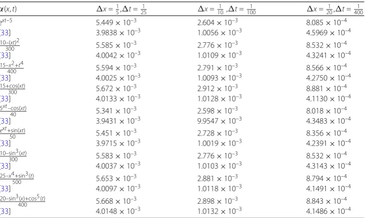
Figure 1Numerical solution of the variable order fractional reaction–subdiffusion equation atλ= 0 for
x=901,t=1001 , final timeT= 0.02,α(x,t) =10+(xt130)4–(xt)5and the maximum absolute error is 6.973845×10⁻⁵
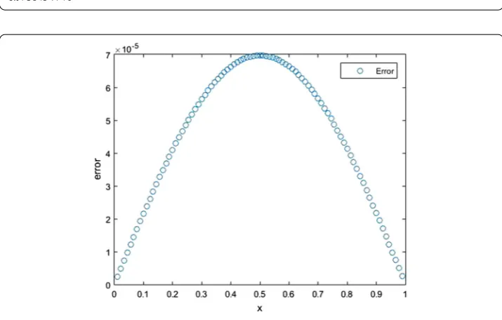
Figure 2Absolute error between the exact and numerical solutions of the variable order fractional reaction–subdiffusion equation atλ= 0 forx= 1
90,t= 1
100, final timeT= 0.02,α(x,t) =
10+(xt)4–(xt)5 130 , and
the maximum absolute error is 6.973845×10⁻⁵
Example 5.2 Consider the following variable-order nonlinear reaction–subdiffusion equation
yt(x,t) =D1–t α(x,t)
yxx(x,t) –y(x,t)
+gx,t,y(x,t), (30)
with the initial and boundary conditions:
y(x, 0) = 0, 0≤x≤1,
Figure 3Numerical solution of the variable order fractional reaction–subdiffusion equation atλ= 0.5 for
x= 1 20,t=
1
200, final timeT= 0.1,α(x,t) = 12–sin3(xt)
12 , and the maximum absolute error is 3.456×10 –3
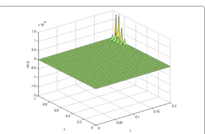
Figure 4Unstable numerical solution of the variable order fractional reaction–subdiffusion equation atλ= 1 forx=401,t=2001 , final timeT= 0.2,α(x,t) =12–sin3(12 xt), the stability condition does not hold
where
gx,t,y(x,t)=y2(x,t) +ext2 –ext3. (31)
The exact solution is
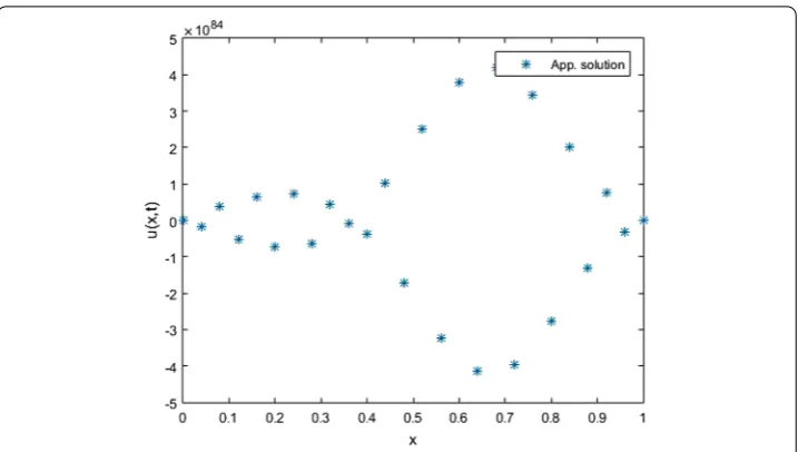
Figure 5Unstable numerical solution of the variable order fractional reaction–subdiffusion equation atλ= 1 forx=251,t=1601 , final timeT= 1,α(x,t) =16+(17xt)5, the stability condition does not hold
Table 2 Dependency of maximum absolute error onx,twithλ= 0,α(x,t) =12–sin123(xt), where the final time isT= 0.1
x t Maximum absolute error
1 10
1
20 3.208×10⁻³
1 10
1
30 2.756×10⁻³
1 20
1
40 2.607×10⁻³
1 30
1
50 2.589×10
–3
1 40
1
50 2.562×10
–3
6 Conclusion and remarks
This paper presents a class of numerical methods for solving the variable order linear and nonlinear reaction–subdiffusion equation. The contribution in this paper is a generaliza-tion of the work done by Sweilam et al. [3]. This class of methods is very close to the weighted average FDM. Special attention is given to the stability of the fractional finite weighted average FDM. For this we have resorted to a kind of fractional John von Neu-mann stability analysis. From the theoretical study we can conclude that this procedure is suitable for the fractional finite weighted average FDM and leads to very good predictions for the stability bounds. The stability of the fractional finite weighted average FDM pre-sented strongly depends on the value of the weighting parameterλ. Numerical solutions and exact solutions of the proposed problem are compared and the derived stability con-dition is checked numerically. From this comparison, we can conclude that the numerical solutions are in excellent agreement with the exact solutions. By comparing the results in this paper with the results in [33], we found that the same order of maximum error was obtained under the same values ofα(x,t),xandt.
All computations in this paper were performed using MATLAB software.
Acknowledgements
Funding
This work is supported by Faculty of Science, Cairo University.
Availability of data and materials
All data and material are available for everyone.
Competing interests
The author declares that he has no competing interests.
Authors’ contributions
The author read and approved the final manuscript.
Publisher’s Note
Springer Nature remains neutral with regard to jurisdictional claims in published maps and institutional affiliations.
Received: 4 April 2018 Accepted: 23 October 2018 References
1. Bagley, R.L., Calico, R.A.: Fractional-order state equations for the control of viscoelastic damped structures. J. Guid. Control Dyn.14(2), 304–311 (1999)
2. Cuesta, E., Finat, J.: Image processing by means of a linear integro-differential equations. In: International Association of Science and Technology for Development, Spain, pp. 438–442 (2003)
3. Sweilam, N.H., Khader, M.M., Adel, M.: Weighted average finite difference methods for fractional reaction-subdiffusion equation. Walailak J. Sci. Technol.11(4), 361–377 (2014)
4. Podlubny, I.: Fractional Differential Equations. Academic Press, San Diego (1999)
5. Abdelhameed, W., Youssri, Y.H.: Generalized Lucas polynomial sequence approach for fractional differential equations. Nonlinear Dyn.89(2), 1341–1355 (2017)
6. Doha, E., Abdelhameed, W., Elkot, N., Youssri, Y.H.: Integral spectral Tchebyshev approach for solving space Riemann–Liouville and Riesz fractional advection–dispersion problems. Adv. Differ. Equ.2017, 284 (2017) 7. Hu, X., Liao, H.L., Liu, F., Turner, I.: A center box method for radially symmetric solution of fractional subdiffusion
equation. Appl. Math. Comput.257, 467–486 (2015)
8. Sweilam, N.H., Khader, M.M., Adel, M.: Numerical simulation of fractional cable equation of spiny neuronal dendrites. J. Adv. Res. (JAR)5, 253–259 (2014)
9. Zheng, M., Liu, F., Liu, Q., Burrage, K., Simpson, M.J.: Numerical solution of the time fractional reaction–diffusion equation with a moving boundary. J. Comput. Phys.338, 493–510 (2017)
10. Sweilam, N.H., Khader, M.M., Al-Bar, R.F.: Numerical studies for a multi-order fractional differential equation. Phys. Lett. A371, 26–33 (2007)
11. Khader, M.M.: Introducing an efficient modification of the homotopy perturbation method by using Chebyshev polynomials. Arab J. Math. Sci.18, 61–71 (2012)
12. Yu, Q., Liu, F., Anh, V., Turner, I.: Solving linear and nonlinear space-time fractional reaction-diffusion equations by Adomian decomposition method. Int. J. Numer. Methods Eng.47(1), 138–153 (2008)
13. Hashim, I., Abdulaziz, O., Momani, S.: Homotopy analysis method for fractional IVPs. Commun. Nonlinear Sci. Numer. Simul.14, 674–684 (2009)
14. Khader, M.M., Adel, M.: Numerical solutions of fractional wave equations using an efficient class of FDM based on the Hermite formula. Adv. Differ. Equ. (2012).https://doi.org/10.1186/s13662-015-0731-0
15. Sweilam, N.H., Khader, M.M., Adel, M.: On the stability analysis of weighted average finite difference methods for fractional wave equation. Fract. Differ. Calc.2(1), 17–29 (2012)
16. Chen, C.M., Liu, F., Anh, V., Turner, I.: Numerical schemes with high spatial accuracy for a variable-order anomalous sub-diffusion equation. SIAM J. Sci. Comput.32(4), 1740–1760 (2010)
17. Chen, C.M., Liu, F., Anh, V., Turner, I.: Numerical simulation for the variable-order Galilei invariant advection diffusion equation with a nonlinear source term. Appl. Math. Comput.217, 5729–5742 (2011)
18. Lin, R., Liu, F., Anh, V., Turner, I.: Stability and convergence of a new explicit finite-difference approximation for the variable-order nonlinear fractional diffusion equation. Appl. Math. Comput.212, 435–445 (2009)
19. Sweilam, N.H., Adel, M., Saadallah, A.F., Soliman, T.M.: Numerical studies for variable order linear and nonlinear fractional cable equation. J. Comput. Theor. Nanosci.12, 1–8 (2015)
20. Zhuang, P., Liu, F., Anh, V., Turner, I.: Numerical methods for the variable-order fractional advection–diffusion equation with a nonlinear source term. SIAM J. Numer. Anal.47, 1760–1781 (2009)
21. Seki, K., Wojcik, M., Tachiya, M.: Fractional reaction–diffusion equation. J. Chem. Phys.119, 2165–2174 (2003) 22. Yuste, S.B., Acedo, L., Lindenberg, K.: Reaction front in anA+B→Creaction–subdiffusion process. Phys. Rev. E69,
036126 (2004)
23. Gorenflo, R., Mainardi, F.: Random walk models for space-fractional diffusion processes. Fract. Calc. Appl. Anal.1, 167–191 (1998)
24. Liu, Q., Liu, F., Turner, I., Anh, V.: Approximation of the Lévy–Feller advection–dispersion process by random walk and finite difference method. J. Comput. Phys.222, 57–70 (2007)
25. Liu, F., Zhuang, P., Anh, V., Turner, I., Burrage, K.: Stability and convergence of the difference methods for the space-time fractional advection–diffusion equation. Appl. Math. Comput.191(1), 12–20 (2007)
26. Zhuang, P., Liu, F.: Implicit difference approximation for the time fractional diffusion equation. J. Appl. Math. Comput.
22(3), 87–99 (2006)
28. Morton, K.W., Mayers, D.F.: Numerical Solution of Partial Differential Equations. Cambridge University Press, Cambridge (1994)
29. Lubich, C.: Discretized fractional calculus. SIAM J. Numer. Anal.17, 704–719 (1986)
30. Yuste, S.B., Acedo, L.: An explicit finite difference method and a new von Neumann-type stability analysis for fractional diffusion equations. SIAM J. Numer. Anal.42, 1862–1874 (2005)
31. Farebrother, R.W.: Linear Least Square Computations. Marcel Dekker, New York (1988)
32. Chang Chen, M., Liu, F., Turner, I., Anh, V.: A Fourier method for the fractional diffusion equation describing sub-diffusion. J. Comput. Phys.227(2), 886–897 (2007)