Algorithms and Arithmetic Operators for
Computing the
η
T
Pairing in Characteristic Three
Jean-Luc Beuchat, Nicolas Brisebarre, J´er´emie Detrey, Eiji Okamoto, Masaaki Shirase, and Tsuyoshi Takagi
Abstract— Since their introduction in constructive crypto-graphic applications, pairings over (hyper)elliptic curves are at the heart of an ever increasing number of protocols. Software implementations being rather slow, the study of hardware archi-tectures became an active research area.
In this paper, we discuss several algorithms to compute theηT pairing in characteristic three and suggest further improvements. These algorithms involve addition, multiplication, cubing, inver-sion, and sometimes cube root extraction overF3m. We propose
a hardware accelerator based on a unified arithmetic operator able to perform the operations required by a given algorithm. We describe the implementation of a compact coprocessor for the fieldF397 given byF3[x]/(x97+x12+ 2), which compares
favorably with other solutions described in the open literature. Index Terms—ηT pairing, finite field arithmetic, elliptic curve, hardware accelerator, FPGA.
I. INTRODUCTION
In 2001, Boneh, Lynn & Shacham [1] proposed a remarkable short signature scheme whose principle is the following. They consider an additive group G1 = hPi of prime order q and a
map-to-point hash functionH:{0,1}∗→G1. The secret key is
an elementxof{1,2, . . . , q−1}and the public key isxP ∈G1
for a signer. Let m ∈ {0,1}∗ be a message, they compute the signature xH(m). To do the verification, they use a map called bilinear pairing that we now define.
Let G1 = hPi be an additive group and G2 a
multiplicati-ve group with identity1. We assume that the discrete logarithm problem is hard in bothG1andG2. A bilinear pairing on(G1, G2)
is a mape:G1×G1→G2that satisfies the following conditions:
1) Bilinearity.For allQ,R,S∈G1,
e(Q+R, S) =e(Q, S)e(R, S) and
e(Q, R+S) =e(Q, R)e(Q, S).
2) Non-degeneracy.e(P, P)6= 1.
3) Computability.e can be efficiently computed.
Modifications of the Weil and Tate pairings provide such maps. The verification in the BLS scheme is done by checking if the valuese(P, xH(m)) ande(xP, H(m))coincide. Actually, if
x0∈ {1,2, . . . , q−1}satisfiese(xP, H(m)) =e(P, x0H(m)), then we obtaine(P, H(m))x=e(P, H(m))x0 thanks to the bilinearity property of the pairing. From the non-degeneracy of the pairing
J.-L. Beuchat and E. Okamoto are with the Graduate School of Systems and Information Engineering, University of Tsukuba, 1-1-1 Tennodai, Tsukuba, Ibaraki, 305-8573, Japan.
N. Brisebarre is with Laboratoire LIP/Ar´enaire (CNRS – ENS Lyon – INRIA – UCBL), ENS Lyon, 46, all´ee d’Italie, F-69364 Lyon Cedex 07, France.
J. Detrey is with the Cosec group, B-IT (Bonn-Aachen International Center for Information Technology), Dahlmannstraße 2, D-53113 Bonn, Germany.
M. Shirase and T. Takagi are with the School of Systems Information Science, Future University-Hakodate, 116-2 Kamedanakano-cho, Hakodate, Hokkaido, 041-8655, Japan.
we know that e(P, H(m))x=e(P, H(m))x0 impliesx=x0. The total cost is one hashing operation, one modular exponentiation and two pairing computations and the signature is twice as short as the one in DSA for similar level of security.
A. Pairings in Cryptology
Pairings were first introduced in cryptology by Menezes, Okamoto & Vanstone [2] and Frey & R¨uck [3] for code-breaking purposes. Mitsunari, Sakai & Kasahara [4] and Sakai, Oghishi & Kasahara [5] seem to be the first to have discovered their constructive properties. Since the foundational work of Joux [6], an already large and ever increasing number of pairing-based protocols has been found. Most of them are described in the survey by Dutta, Barua & Sarkar [7]. As noticed in that survey, such protocols rely critically on efficient algorithms and imple-mentations of pairing primitives.
According to [8], [9], when dealing with general curves pro-viding common levels of security, the Tate pairing seems to be more efficient for computation than the Weil pairing and we now describe it.
Let E be a supersingular1 elliptic curve over Fpm, where p is a prime and m a positive integer, and let E(Fpm) denote the group of its points. Let ` > 0 be an integer relatively prime to p. The embedding degree (or security multiplier) is the least positive integer k satisfying pkm ≡ 1 (mod`). Let
E(Fpm)[`]denote the`-torsion subgroup ofE(Fpm),i.e. the set of elements P ofE(Fpm)that satisfy [`]P =O, where Ois the point at infinity of the elliptic curve. Let P ∈ E(Fpm)[`] and
Q ∈ E(Fpkm)[`], let f`,P be a rational function on the curve with divisor `(P)−`(O) (see [10] for an account of divisors), there exists a divisorDQ equivalent to(Q)−(O), with a support disjoint from the support off`,P. Then the Tate pairing2of order ` is the map e : E(Fpm)[`]×E(Fpkm)[`] → F∗pkm defined by
e(P, Q) =f`,P(DQ)(p km−1)/`
. The kind of powering that occurs in this definition is called the final exponentiation; it makes it possible to get values in a multiplicative subgroup ofF∗pkm(which is required by most of the cryptographic applications) instead of a multiplicative subgroup of a quotient ofF∗pkm.
In [11], Barretoet al.proved that this pairing can be computed as e(P, Q) = f`,P(Q)
pkm−1
` , where f`,P is evaluated on a point rather than on a divisor. Thanks to a distortion map ψ : E(Fpm)[`]→E(Fpkm)[`] (the concept of a distortion map was introduced in [12]), one can define the modified Tate pairing ˆe
by ˆe(P, Q) =e(P, ψ(Q))for allP, Q∈E(Fpm)[`].
Miller [13], [14] proposed in 1986 the first algorithm for com-puting Weil and Tate pairings. Different ways for comcom-puting the
1See Theorem V.3.1 of [10] for a definition.
Tate pairing can be found in [11], [15]–[17]. In [18], Barretoet al.introduced theηT pairing which extended and improved the Duursma-Lee techniques [16]. It makes it possible to efficiently compute the Tate pairing. TheηT pairing is presented in Section II in which we recall the relation between it and the modified Tate pairing.
B. Implementation Challenges
The software implementations of these successive algorithmic improvements being rather slow, the need for fine hardware implementations is strong. This is a critical issue to make pairings popular and of common use in cryptography and in particular in view of a successful industrial transfer. The papers [19]–[27] address that problem.
In this paper, we deal with the characteristic three case and, given a positive integer m coprime to 6, we consider E, a supersingular elliptic curve over F3m, defined by the equation
y2=x3−x+b, withb∈ {−1,1}. Following the discussion at the beginning of Section 5 of [18], there is no loss of generality from considering this case since these curves offer the same level of security for pairing applications as any supersingular elliptic curve overF3m. The considered curve has an embedding degree of6, which is the maximum value possible for supersingular elliptic curves, and hence seems to be an attractive choice for pairing implementation.
C. Our Contribution
The algorithm given in [18] for computing the ηT pairing halves the number of iterations used in the approach by Duursma & Lee [16] but has the drawback of using inverse Frobenius maps. In [25] Beuchat et al. proposed a modified ηT pairing algorithm in characteristic three that does not require any inverse Frobenius map. Moreover, they designed a novel arithmetic operator implementing addition, cubing, and multiplication over
F397 which performs in a fast and cheap way the step of final
exponentiation [26]. Then they extended in [27] this approach to the computation of the reducedηT pairing (i.e. the combination of theηT pairing and the final exponentiation).
In this article, we present a synthesis and an improvement of the results of the papers [25]–[27]. The outline of the paper is the following. In Section II, we define theηT pairing and its reduced form, we give different algorithms to compute them and we provide exact cost evaluations for these algorithms. Section III is dedicated to the presentation of a reducedηT pairing coprocessor that is based on a unified arithmetic operator that implements the various required elementary operations over F3m. We want to mention that all the material (i.e. algorithms and architectures) presented in this section can be easily adapted to work on any field
Fp[x]/(f(x))for any prime pand any polynomial f irreducible
over Fp. We implemented our coprocessor on several Field-Programmable Gate Array (FPGA) families for the field F397
given by F3[x]/(x97 +x12 + 2). We provide the reader with
a comprehensive comparison against state-of-the-art ηT pairing accelerators in Section IV and conclude our article in Section V.
II. COMPUTATION OF THEηT PAIRING INCHARACTERISTIC THREE
A. Preliminary Definitions
We use here the definition of theηT pairing as introduced by Barreto et al. in [18]. The interested reader shall find in that
article all the details related to the mathematical construction of the pairing, which we will deliberately not mention here for clarity’s sake.
Let E be the supersingular elliptic curve defined by the equation E :y2 =x3−x+b, where b∈ {−1,1}. Considering a positive integer mcoprime to6, the number of rational points of E over the finite field F3m is given by N = #E(F3m) = 3m+ 1 +µb3m2+1, with
µ=
+1 ifm≡1,11 (mod 12), or
−1 ifm≡5,7 (mod 12).
The embedding degreek ofE is then6.
Choosing T = 3m−N = −µb3m2+1 −1 and an integer `
dividing N, we define theηT pairing of two points P andQof the `-torsion E(F3m)[`]as
ηT(P, Q) =
fT ,P(ψ(Q)) ifT >0(i.e.µb=−1), or f−T ,−P(ψ(Q)) ifT <0(i.e.µb= 1), where:
• ψis a distortion map fromE(F3m)[`]toE(F36m)[`]defined asψ(x, y) = (ρ−x, yσ)for all(x, y)∈E(F3m)[`], as given in [11], where ρandσare elements ofF36m satisfying the equations ρ3−ρ−b= 0 andσ2+ 1 = 0.
As already remarked in [20], this allows for repre-senting F36m as an extension of F3m using the basis (1, σ, ρ, σρ, ρ2, σρ2):F36m =F3m[σ, ρ]∼=F3m[X, Y]/(X2+ 1, Y3−Y −b). Hence, all the computations overF36m can be replaced by computations overF3m, as explicitly shown in Appendices V and VI.
• fn,P, forn∈NandP ∈E(F3m)[`], is a rational function defined over E(F36m)[`] with divisor (fn,P) = n(P)− ([n]P)−(n−1)(O).
In order to ensure that the obtained pairing values belong to the group of the `th roots of unity ofF∗36m, we actually have to compute the reducedηT pairing, defined as ηT(P, Q)M, where
M= 3
6m− 1
N =
“
33m−1”`
3m+ 1´“
3m+ 1−µb3m+12 ”
.
In the following, we will refer to this additional step as final exponentiation.
One should also note that, in characteristic 3, we have the following relation between the reduced ηT and modified Tate pairings:
“
ηT(P, Q)M
”3T2 =
“
ˆ e(P, Q)M
”L
,
withL=−µb3m2+3. Using vas a shorthand forηT(P, Q)M, we
can compute the modified Tate pairing according to the following formula:
ˆ
e(P, Q)M =v−2 v3
m+1 2 3
mq
v3m−21 !−µb
.
Noting T0 = −µbT = 3m2+1 +µb and P0 = [−µb]P, we
now have to computeηT(P, Q)M =fT0,P0(ψ(Q))M. Using the
Duursma-Lee techniques [16] to simplify the computation offn,P in Miller’s algorithm, we obtain
fT0,P0(ψ(Q)) = 0
B @
m−1 2 Y
i=0
g[3i]P0(ψ(Q))3
m−1 2 −i
1
C
where:
• gV, for allV = (xV, yV)∈E(F3m)[`], is the rational func-tion introduced by Duursma and Lee in [16], defined over
E(F36m)[`] and having divisor (gV) = 3(V) + ([−3]V)− 4(O). For all(x, y)∈E(F36m)[`], we have
gV(x, y) =yV3y−(x3V −x+b)2.
• lV, for allV = (xV, yV)∈E(F3m)[`], is the equation of the line corresponding to the addition ofh3m2+1
i
V with[µb]V, defined for all(x, y)∈E(F36m)[`]:
lV(x, y) =y−λyV(x−xV)−µbyV,
with
λ= (−1)m+12 =
+1 ifm≡7,11 (mod 12), or
−1 ifm≡1,5 (mod 12).
We can also rewrite the equation oflV as
lV(x, y) =y+λyV(xV −x−νb),
introducing
ν=µλ=
+1 ifm≡5,11 (mod 12), or
−1 ifm≡1,7 (mod 12).
The remaining of this section will present and discuss various algorithms that can be used to effectively compute the reducedηT pairing. The next three subsections will focus on the computation of ηT(P, Q) only, the details of the final exponentiation being given in Section II-E. Finally, cost evaluations and comparisons will be presented in Section II-F.
B. Direct Approaches
1) Direct Algorithm: From the expression of fT0,P0, noting
˜
Q=ψ(Q), we can write
fT0,P0( ˜Q) = „
. . .“gP0( ˜Q)3·g[3]P0( ˜Q) ”3
. . .
«3
g» 3m−21
–
P0( ˜Q)·lP0( ˜Q).
Noting P0 = (xP0, yP0) andQ= (xQ, yQ), we have[3i]P0 = “
x3P20i−ib,(−1)iy3 2i P0
”
andQ˜=ψ(Q) = (ρ−xQ, yQσ). Injecting these in the expressions of g[3i]P0 and lP0 and defining m0 =
m−1
2 , we obtain
g[3i]P0( ˜Q) =
(−1)iyP320i+1yQσ−
“
x3P20i+1+xQ+ (1−i)b−ρ
”2
, and
lP0( ˜Q) =
yQσ−(−1)m
0 y32m
0+1
P0 „
x32m 0+1
P0 +xQ+ (1−m0)b−ρ
«
.
An iterative implementation of the ηT pairing following this construction is given in Algorithm 1. The cost of each pseudo-code instruction is given as comments in terms of addi-tions/subtractions (A), multiplications (M) and cubings (C) over the underlying fieldF3m.
A few remarks concerning this algorithm:
• The multiplication by−µbon line 1 is for free. Indeed,−µb
being a constant (1or−1) for fixedm andb, one can just compute the value of−µbwhen those parameters are chosen, and propagate sign corrections onyP throughout the whole algorithm.
Algorithm 1Direct algorithm for computing theηT pairing. Input: P, Q∈E(F3m)[`].
Output: ηT(P, Q)∈F∗36m. 1. yP ← −µbyP;
2. xP ←x3P; yP←y3P; (2C) 3. t←xP+xQ+b; u←yPyQ; (1M,2A) 4. R←(−t2+uσ−tρ−ρ2)3; (1M,2C,3A) 5. xP ←x9P; yP← −y9P; (4C) 6. t←xP+xQ; u←yPyQ; (1M,1A) 7. S← −t2+uσ−tρ−ρ2; (1M)
8. R←R·S; (6M,21A)
9. fori←2to m2−1 do
10. R←R3; (6C,6A)
11. xP←x9P−b; yP← −y9P; (4C,1A) 12. t←xP+xQ; u←yPyQ; (1M,1A) 13. S← −t2+uσ−tρ−ρ2; (1M) 14. R←R·S; (12M,59A) 15. end for
16. S← −yPt+yQσ+yPρ; (1M) 17. R←R·S; (12M,51A) 18. returnR;
• Similarly, multiplications by λ, ν and b do not have any impact on the cost of the algorithm. The value of these constants are known in advance, and actually only represent sign changes in the algorithm.
• Since the representation of−t2+uσ−tρ−ρ2as an element of the tower fieldF36m is sparse, the cubing on line 4 involves only 1multiplication, 2cubings and 3additions over F3m, as detailed in Appendix V-B.
• Additionally,(−t2+uσ−tρ−ρ2)3has the same sparsity, and therefore the product ofRandS on line 8 can be computed by means of only 6 multiplications and 21 additions over
F3m, as per Appendix VI-C.
• Inside the loop, the cubing ofR on line 10 is computed in 6cubings and6additions overF3m (Appendix V-A).
• The multiplication of R by S on line 14 involves only 12 multiplications and 59 additions over F3m, as S is sparse (Appendix VI-B).
• The final product on line 17 is in turn computed by means of 12 multiplications and 51 additions, also thanks to the sparsity ofS, as detailed in Appendix VI-B.
2) Simplification using Cube Roots: Cubing the intermediate result R ∈ F∗36m at each iteration of Algorithm 1 is quite expensive. But one can use the fact that, due to the bilinearity of the reducedηT pairing,
ηT(P, Q)M =
0
@ηT
“
P,h3−m−21 i
Q
”3m2−1 1
A
M ,
to compute instead
fT0,P0( ˜Q)3
m−1 2
=
0
B @
m−1 2 Y
i=0
g[3i]P0( ˜Q)3
m−1−i
1
C AlP0( ˜Q)
3m−21
,
with Q˜=ψ“h3−m2−1 i
Q”=“ρ−x3Q−(ν+ 1)b,−λy3Qσ
”
Expanding everything, we obtain the following expressions, again withm0=m2−1:
g[3i]P0( ˜Q)3
m−1−i =
−λy3Pi0y3 −i
Q σ−
“
x3Pi0+x3 −i
Q −νb−ρ
”2
, and
lP0( ˜Q)3
m−1 2
=y3−m 0
Q σ+λy
3m0 P0
„
x3m 0
P0 +x3 −m0
Q −νb−ρ
«
.
This naturally gives another iterative method to compute
ηT(P, Q), presented in Algorithm 2. Here, the cubings overF36m are traded for cube roots (noted R) over F3m, which can be efficiently computed by means of a specific operator (see III-E for further details).
Algorithm 2Simplified algorithm for computing theηT pairing, with cube roots.
Input: P, Q∈E(F3m)[`]. Output: ηT(P, Q)∈F∗36m.
1. xP ←xP−νb; (1A)
2. yP ← −µbyP;
3. t←xP+xQ; u←yPyQ; (1M, 1A) 4. R← −t2−λuσ−tρ−ρ2; (1M) 5. xP ←x3P; yP ←yP3; (2C) 6. xQ←√3xQ; yQ←√3yQ; (2R)
7. t←xP+xQ; u←yPyQ; (1M, 1A) 8. S← −t2−λuσ−tρ−ρ2; (1M)
9. R←R·S; (6M,21A)
10. fori←2to m2−1 do
11. xP ←x3P; yP ←y3P; (2C) 12. xQ←√3xQ; yQ←√3yQ; (2R)
13. t←xP+xQ; u←yPyQ; (1M, 1A) 14. S← −t2−λuσ−tρ−ρ2; (1M) 15. R←R·S; (12M,59A) 16. end for
17. S←λyPt+yQσ−λyPρ; (1M) 18. R←R·S; (12M,51A) 19. returnR;
3) Tabulating the Cube Roots: Even if cube roots can be computed with only a slight hardware overhead, it is sometimes advisable to restrict the hardware complexity of the arithmetic unit in order to achieve higher clock frequencies. The previous algorithm can easily be adapted to cube-root-free coprocessors by simply noticing that, as xQ and yQ ∈F3m,x3
−i Q =x3
m−i
Q and
y3Q−i =y3Qm−i.
Therefore, computing them−1successive cubings ofxQ and yQ, it is possible to tabulate the pre-computed values ofx3
−i
Q and
y3Q−i which will be looked-up on lines 6 and 12 of Algorithm 2 instead of computing the actual cube roots.
The m−1 cube roots of Algorithm 2 are hence traded for 2m−2cubings, at the expense of extra registers required to store the tabulated values asm−1elements ofF3m.
This idea, originally suggested by Barretoet al.[18], was for instance applied by Ronan et al. in [23] in the case m ≡ 1 (mod 12), although they curiously do not compute the actualηT pairing, but the value
ηT
“
P,[3−m]Q
”3m2−1
=ηT(P, Q)3
−m2+1
.
C. Reversed-Loop Approaches
In [18], Barreto et al.suggest reversing the loop to compute the ηT pairing. To that purpose, they introduce a new indexj= 3m−21 −ifor the loop. TakingQ˜=ψ(Q), we find
fT0,P0( ˜Q) =lP0( ˜Q) 0
B @
m−1 2 Y
j=0
g» 3m2−1−j
– P0( ˜Q)
3j 1
C A.
1) Reversed-Loop Algorithm:Directly injecting the expression of h3m2−1−j
i
P0 = “x3P−02j−1−(ν+ 1−j)b,−λ(−1)jy3 −2j−1 P0
”
into the formulas, we obtain
lP0( ˜Q) =yQσ+λyP0`xP0+xQ−νb−ρ´, and
g» 3m2−1−j
– P0( ˜Q)
3j
=
−λy3P−0jy3
j Qσ−
“
x3P−0j+x3
j
Q −νb−ρ
”2
.
Following this expression, a third iterative scheme for com-puting the ηT pairing can be directly devised, as detailed in Algorithm 3. In the casem≡1 (mod 12), this is the exact same algorithm as described by Barretoet al.in [18].
Algorithm 3 Reversed-loop algorithm for computing the ηT pairing, with cube roots.
Input: P, Q∈E(F3m)[`]. Output: ηT(P, Q)∈F∗36m.
1. xP ←xP−νb; (1A)
2. yP ← −µbyP;
3. t←xP+xQ; (1A)
4. R←(λyPt+yQσ−λyPρ)·(−t2−λyPyQσ−tρ−ρ2); (6M,1C,6A)
5. forj←1to m−21 do 6. xP← 3
√
xP; yP← 3
√
yP; (2R)
7. xQ←x3Q; yQ←y3Q; (2C) 8. t←xP+xQ; u←yPyQ; (1M,1A) 9. S← −t2−λuσ−tρ−ρ2; (1M) 10. R←R·S; (12M,59A) 11. end for
12. returnR;
It is to be noted that given the expression of its operands, the multiplication on line 4 is computed by means of only 6 multiplications,1cubing and6additions overF3m, as described in Appendix VI-D.
As for Algorithm 2, Algorithm 3 also requires the computation of cube roots. A similar technique of pre-computation and tabu-lation of the cube roots thanks to successive cubings ofxP and yP can be also be used, although we will not detail it here.
2) Eliminating the Cube Roots: The apparent duality between Algorithms 2 and 3 can be exploited to find another cube-free algorithm, still based on the reversed loop but similar to Algorithm 1.
For that purpose, we once again compute the reduced ηT pairing ofP andQas
ηT(P, Q)M =
0
@ηT
“
P,
h
3−m
−1 2
i
Q
”3m2−1 1
A
NotingQ˜=ψ
“h
3−m2−1 i
Q
”
, the reversed loop becomes
fT0,P0( ˜Q)3
m−1 2
=lP0( ˜Q)3
m−1 2
0
B @
m−1 2 Y
j=0
g» 3m−21−j
– P0( ˜Q)
3m2−1+j 1
C A
=lP0( ˜Q)3
m−1 2
0
B @
m−1 2 Y
j=0
hj,P0( ˜Q)3
m−1 2 −j
1
C A
= . . .
„ “
lP0( ˜Q)·h0,P0( ˜Q) ”3
h1,P0( ˜Q) «3
. . .
!3
hm−1 2 ,P0
( ˜Q),
with the rational functionhj,P0( ˜Q)defined as
hj,P0( ˜Q) =g» 3m2−1−j
– P0( ˜Q)
32j .
We then compute the explicit expressions of lP( ˜Q) and hj,P0( ˜Q):
lP0( ˜Q) =−λyQ3σ+λyP0 “
xP0+x3Q+b−ρ ”
, and
hj,P0( ˜Q) =
(−1)jyP0y3 2j+1
Q σ−
“
xP0+x3 2j+1
Q + (1−j)b−ρ
”2
.
Algorithm 4 is a direct implementation of the previous com-putation of ηT(P, Q). Similarly to Algorithm 1, it uses cubings over F36m in order to avoid the cube roots of Algorithm 3. In the casem≡1 (mod 12), this algorithm corresponds to the ηT pairing computation described by Beuchatet al.in [25]. Algorithm 4Cube-root-free reversed-loop algorithm for comput-ing theηT pairing.
Input: P, Q∈E(F3m)[`]. Output: ηT(P, Q)∈F∗36m.
1. xP ←xP+b; (1A)
2. yP ← −µbyP;
3. xQ←x3Q; yQ←y3Q; (2C)
4. t←xP+xQ; (1A)
5. R←(λyPt−λyQσ−λyPρ)·(−t2+yPyQσ−tρ−ρ2); (6M,1C,6A)
6. forj←1to m2−1 do
7. R←R3; (6C,6A)
8. xQ←x9Q−b; yQ← −y9Q; (4C,1A) 9. t←xP+xQ; u←yPyQ; (1M, 1A) 10. S← −t2+uσ−tρ−ρ2; (1M) 11. R←R·S; (12M,59A) 12. end for
13. returnR;
D. Loop Unrolling
Grangeret al.[28] proposed a loop unrolling technique for the Duursma-Lee algorithm. They exploit the sparsity ofgV in order to reduce the number of multiplications overF3m, exactly in the same way as we reduced the first two iterations of Algorithms 1 and 2.
By noting that hj,P0( ˜Q)3 is also as sparse as hj,P0( ˜Q) (see
Appendix V-B for details), we can apply the same approach to Algorithm 4.
In two successive iterations2j0−1 and2j0 of the loop, for 1≤j0≤ bm−41c, we compute the new value ofR as
R←“R3·h2j0−1,P0( ˜Q) ”3
·h2j0,P0( ˜Q)
= R9·h2j0−1,P0( ˜Q)3·h2j0,P0( ˜Q).
The values of h2j0−1,P0( ˜Q) and h2j0,P0( ˜Q), computed at
iterations 2j0 −1 and 2j0 respectively, are both of the form
−t2+uσ−tρ−ρ2. Therefore, givent andu, the computation of h2j0−1,P0( ˜Q)3 requires only 1multiplication, 2cubings and
3 additions over F3m, as per Appendix V-B. Similarly, the product of h2j0−1,P0( ˜Q)3 and h2j0,P0( ˜Q) can be computed by
means of only6multiplications and21additions, as explained in Appendix VI-C. Finally, multiplying this product byR9requires a full F36m multiplication, which can be performed with 15 multiplications and 67additions overF3m (see Appendix VI-A). Hence, the cost of such a double iteration would be of 25 multiplications (neglecting the other operations), whereas two iterations of the original loop from Algorithm 4 cost2×14 = 28 multiplications.
Following this, we can unroll the main loop of Algorithm 4 in order to save multiplications by computing two iterations at a time. The resulting scheme is shown in Algorithm 5, for the case wherem2−1is even. Ifm2−1is actually odd, one just has to restrict the loop on j0 from1to m4−3, and compute the last product by an extra iteration of the original loop, for the additional cost of 14multiplications,10cubings and68additions overF3m.
Algorithm 5Unrolled loop for the computation of theηT pairing when m2−1 is even.
Input: P, Q∈E(F3m)[`]. Output: ηT(P, Q)∈F∗36m.
1. xP ←xP+b; (1A)
2. yP ← −µbyP;
3. xQ←x3Q; yQ←yQ3; (2C)
4. t←xP+xQ; (1A)
5. R←(λyPt−λyQσ−λyPρ)·(−t2+yPyQσ−tρ−ρ2); (6M,1C,6A)
6. forj0←1to m−41 do
7. R←R9; (12C,12A)
8. xQ←x9Q−b; yQ←yQ9; (4C,1A) 9. t←xP+xQ; u←yPyQ; (1M,1A) 10. S←(−t2−uσ−tρ−ρ2)3; (1M,2C,3A) 11. xQ←x9Q−b; yQ←yQ9; (4C,1A) 12. t←xP+xQ; u←yPyQ; (1M,1A) 13. S0← −t2+uσ−tρ−ρ2; (1M) 14. S←S·S0; (6M,21A) 15. R←R·S; (15M,67A) 16. end for
17. returnR;
It is to be noted that one could also straightforwardly apply a similar loop unrolling technique to Algorithm 1. However, we will not detail this point any further, for it is rigourously identical to the previous case.
E. Final Exponentiation
`th powers. This reduction is achieved by means of a final exponentiation, in which ηT(P, Q) is raised to the Mth power, with
M =“33m−1”`
3m+ 1´“
3m+ 1−µb3m2+1 ”
.
For this particular exponentiation, we use the scheme presented by Shiraseet al.in [29].
Taking U = ηT(P, Q) ∈ F∗36m, we first compute U3 3m−1
. Writing U as U0+U1σ, where U0 and U1 ∈F∗33m, and seeing that
U33m =U0−U1σ, and
U−1 = U0−U1σ U02+U12 ,
we obtain the following expression forU33m−1:
U33m−1=(U
2
0−U12) +U0U1σ
U2 0+U12
.
This computation is directly implemented in Algorithm 6, where the multiplication (line 3), the squarings (lines 1 and 2), and the inversion (line 5) over F33m are performed following the algorithms presented in Appendices II, III and IV respectively.
Algorithm 6Computation ofU33m−1 inF∗36m.
Input: U=u0+u1σ+u2ρ+u3σρ+u4ρ2+u5σρ2∈F∗36m. Output: V =U33m−1∈T2(F33m).
1. m0←(u0+u2ρ+u4ρ2)2; (5M, 7A)
2. m1←(u1+u3ρ+u5ρ2)2; (5M, 7A)
3. m2←(u0+u2ρ+u4ρ2)·(u1+u3ρ+u5ρ2); (6M,12A)
4. a0←m0−m1;a1←m0+m1; (6A)
5. i←a−11; (12M, 11A,1I) 6. V0←a0·i; (6M,12A)
7. V1←m2·i; (6M,12A)
8. returnV0+V1σ;
One can then remark that
(U02−U12)2+ (U0U1)2
(U02+U12)2 = 1,
meaning that U33m−1 is in fact an element ofT2(F33m), where
T2(F33m) ={X0+X1σ ∈ F∗36m : X02+X12 = 1} is the torus
as introduced by Grangeret al. for the case of the Tate pairing in [28].
This is a crucial point here, since arithmetic on the torus
T2(F33m)is much simpler than arithmetic onF∗36m. Thus, given
U ∈T2(F33m), Algorithm 7 computes U3 m+1
in only 9 multi-plications and18or19(depending on the value ofmmodulo6) additions overF3m.
Finally, Algorithm 8 implements the complete final exponenti-ation. GivenU∈F∗36m as input, it first computesU3
3m−1 thanks to Algorithm 6, then calls Algorithm 7 to obtainU(33m−1)(3m+1). Then W =U(33m−1)(3m+1)3(m+1)/2 is computed by successive cubings over F36m, while V = U(3
3m−1)(3m+1)(3m+1) is ob-tained by a second call to Algorithm 7. The value to be computed is then
UM =
V ·W−1 whenµb= 1, or
V ·W whenµb=−1,
hence the computation ofW0=W−µbon line 8. Whenµb=−1, this is just a dummy operation, but it is an actual inversion when
Algorithm 7Computation ofU3m+1in the torusT2(F33m).
Input: U =u0+u1σ+u2ρ+u3σρ+u4ρ2+u5σρ2∈T2(F33m). Output: V =U3m+1∈T2(F33m).
1. a0←u0+u1;a1←u2+u3;a2←u4−u5; (3A)
2. m0←u0·u4;m1←u1·u5;m2←u2·u4; (3M)
3. m3←u3·u5;m4←a0·a2;m5←u1·u2; (3M)
4. m6←u0·u3;m7←a0·a1;m8←a1·a2; (3M)
5. a3←m5+m6−m7;a4← −m2−m3; (3A)
6. a5← −m2+m3;a6← −m0+m1+m4; (3A)
7. ifm≡1 (mod 6)then
8. v0←1 +m0+m1+ba4; (3A)
9. v1←bm5−bm6+a6; (2A)
10. v2← −a3+a4; (1A)
11. v3←m8+a5−ba6; (2A)
12. v4← −ba3−ba4; (1A)
13. v5←bm8+ba5; (1A)
14. else ifm≡5 (mod 6)then
15. v0←1 +m0+m1−ba4; (3A)
16. v1← −bm5+bm6+a6; (2A)
17. v2←a3;
18. v3←m8+a5+ba6; (2A)
19. v4← −ba3−ba4; (1A)
20. v5← −bm8−ba5; (1A)
21. end if
22. returnv0+v1σ+v2ρ+v3σρ+v4ρ2+v5σρ2;
µb= 1. However, as W ∈T2(F33m), writing W =W0+W1σ,
we have
W−1= W0−W1σ
W02+W12 =W0−W1σ.
Inversion overT2(F33m)is therefore completely free, as it suffices to propagate the sign corrections in the final product V ·W0, implemented as a full multiplication over F∗36m.
Algorithm 8Final exponentiation of the reducedηT pairing [29]. Input: U =u0+u1σ+u2ρ+u3σρ+u4ρ2+u5σρ2∈F∗36m. Output: UM ∈ T2(F33m) ⊂ F∗36m, with the exponent M =
(33m−1)(3m+ 1)(3m+ 1−µb3m2+1).
1. V ←U33m−1; (40M,67A,1I) 2. V ←V3m+1; (9M, 18or19A) 3. W←V;
4. fori←1to m2+1 do
5. W ←W3; (6C,6A)
6. end for
7. V ←V3m+1; (9M, 18or19A) 8. W0←W−µb;
9. returnV ·W0; (15M,67A)
F. Overall Cost Evaluations and Comparisons
The costs of all the previously detailed algorithms are sum-marized in Table I, in terms of additions (or subtractions), multiplications, cubings, cube roots and inversions over F3m.
TABLE I
COST OF THE PRESENTED ALGORITHMS FOR COMPUTING THEηTPAIRING AND THE FINAL EXPONENTIATION,
IN TERMS OF OPERATIONS OVER THE UNDERLYING FIELDF3m.
Additions Multiplications Cubings Cube roots Inversions
Direct loop No cube root (Algorithm 1) 67 m−1
2 + 11 7m+ 2 5m−7 0 0
With cube roots (Algorithm 2) 30m−15 7m+ 2 m−1 m−1 0
Reversed loop With cube roots (Algorithm 3) 30m−22 7m−1 m m−1 0
No cube root (Algorithm 4) 67m−21+ 8 7m−1 5m−2 0 0
Unrolled loop m2−1 is even 107m4−1+ 8 25m4−1+ 6 11m2−1+ 3 0 0
(Algorithm 5) m−21 is odd 107m−43+ 76 25m4−3+ 20 11m2−1+ 2 0 0
Final exp. m≡1 (mod 6) 3m+ 175 73 3m+ 3 0 1
(Algorithm 8) m≡5 (mod 6) 3m+ 173 73 3m+ 3 0 1
will therefore depend on the practicality of the computation of cube roots in the given finite field F3m (see the discussion in Section III-E).
This table also shows a slight superiority of reversed-loop algorithms versus direct-loop approaches. This is the reason why we chose to apply the loop unrolling technique to Algorithm 4.
The advantage of such a loop unrolling becomes also clearer when looking at Table I. From Algorithm 4 to Algorithm 5, we trade approximately 27m/4 additions and3m/4 multiplications form/2cubings overF3m.
The costs of these algorithms for m= 97, on which we focus more closely in this paper, is given in Table II. As detailed in Section III-B, we can compute the inversion overF397 according
to Fermat’s little theorem in 9 multiplications and 96 cubings, which allows us to express these costs in terms of additions, multiplications, cubings and cube roots only. The total number of operations for the complete computation of the reduced ηT pairing, using Algorithm 5 for the ηT pairing and Algorithm 8 for the final exponentiation, is also given.
TABLE II
COST EVALUATIONS OF THE REDUCEDηTPAIRING FORm= 97. INVERSION OVERF397IS CARRIED OUT ACCORDING TOFERMAT’S
LITTLE THEOREM IN9MULTIPLICATIONS AND96CUBINGS.
A M C R
Direct loop (Algorithm 1)(Algorithm 2) 32272895 681681 47896 960
Reversed loop (Algorithm 3) 2888 678 97 96
(Algorithm 4) 3224 678 483 0 Unrolled loop (Algorithm 5) 2576 606 531 0 Final exp. (Algorithm 8) 466 82 390 0 Total (Algorithms 5 and 8) 3042 688 921 0
III. A COPROCESSOR FORARITHMETIC OVERF3m
The ηT pairing calculation in characteristic 3 requires ad-dition, multiplication, cubing, inversion, and sometimes cube root extraction over F3m. We propose here a unified arithmetic operator which implements the required operations, and describe a hardware accelerator for pairing-based cryptography.
In the following, elements of the field extension F3m will be represented using a polynomial basis. Given a degree-m
irre-ducible polynomialf(x)∈F3[x], we haveF3m ∼=F3[x]/(f(x)). Each element of F3m will then be represented as a polynomial
p(x)of degree(m−1)and coefficients inF3:
p(x) =pm−1xm−1+. . .+p1x+p0.
Several researchers reported implementations of the Tate and
ηT pairings on a supersingular curve defined on the field F397.
Therefore, we discuss the implementation of Algorithm 5 for the field F3[x]/(x97+x12+ 2) and the curvey2 =x3−x+ 1(i.e.
b= 1) on our coprocessor.
It is nonetheless important to note that the architectures and algorithms presented here can be easily adapted to different parameters. For instance a different irreducible polynomialf(x), a different field extension degree m, or even a different char-acteristic p (cubing and cube root extraction, being respectively Frobenius and inverse Frobenius maps in characteristic 3, then replaced by raising to the pth power andpth root extraction).
A. Multiplication overF3m
Three families of algorithms allow one to compute d0(x)·
d1(x) modf(x) (see for instance [30]–[32] for an account of modular multiplication). In parallel-serial schemes, a single co-efficient of the multiplier d0(x) is processed at each step. This leads to small operators performing a multiplication in mclock cycles. Parallel multipliers compute a degree-(2m−2)polynomial and carry out a final modular reduction. They achieve a higher throughput at the price of a larger circuit area. By processingD
coefficients of an operand at each clock cycle, array multipliers, introduced by Song and Parhi in [33], offer a good trade-off between computation time and circuit area and are at the heart of several pairing coprocessors (see for instance [19], [20], [22], [23], [25], [34]).
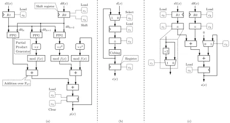
Depending on the order in which coefficients of d0(x) are processed, array multipliers can be implemented according to two schemes: most-significant element (MSE) first and least-significant element (LSE) first. Algorithm 9 summarizes the MSE-first scheme proposed by Shu, Kwon & Gaj [22]. Figure 1a illustrates the architecture of this operator for D = 3. It mainly consists of three Partial Product Generators (PPGs), three modulo
c2
c4 ×x2
PPG
PPG PPG
c5
c1
Generator Product Partial
Addition overF3m
(b) (c)
(a)
d(x)
c(x) Select
Load
Cubing ±
Register 1 0
Shift register d0(x) Load
Shift
d03i+2
Load
Clear
p(x)
d03i d03i+1 R0 R1
d1(x)
Load
c0
c1
c2
c3
c4
c3
c2
c1
c0
± ±
s(x)
d1(x) d0(x)
×2
1 0
0 1 0
Load Load
modf(x) modf(x)
Load modf(x)
×x
R0
×x3
R1
c1
c0
c3
Fig. 1. Arithmetic operators overF3m. (a) Multiplication (D = 3 coefficients of d0(x) are processed at each clock cycle) [22]. (b) Cubing. (c) Addition/subtraction of two operands and accumulation. Boxes with rounded corners involve only wiring. Theci’s denote control bits.
trinomial or a pentanomial, modulo f(x) operations are easy to implement. Consider for instance f(x) = x97 +x12+ 2 and let u(x) = x·d1(x) be a degree-97 polynomial. It suffices to remove u97·f(x) =u97x97+u97x12+ 2u97 fromu(x) to get
u(x) modf(x). This involves only two multiplications and two subtractions overF3, namelyu12−1·u97andu0−2·u97.
Elements ofF3are often represented as2-bit unsigned integers.
Let d0i = 2d0Hi +d0Li and d1j = 2d1Hj +d1Lj. Multiplication overF3={0,1,2}is then defined as follows:
d0i·d1j= 2
“
d0Hi d1Lj ∨d0Lid1Hj
”
+“d0Lid1Lj ∨d0Hi d1Hj
”
,
and can be implemented by means of two4-input Look-Up Tables (LUTs). Sinced0imultiplies all coefficients ofd1, the fanout of our array multiplier is equal to2m.
However, a careful encoding of the elements ofF3can reduce
the fanout of the operator [35]. Since2≡ −1 (mod 3), we take advantage of the borrow-save system [36] in order to represent the elements ofF3={0,1,−1}:d0iis encoded by a positive bitd0+i and a negative bitd0−i such thatd0i=d0+i −d0
−
i . Multiplication overF3 is now defined by:
d0i·d1j =
“
(1−d1−j)d1+jd0+i ∨d1−j(1−d1+j)(1−d0+i )”−
“
(1−d1−j)d1+jd0−i ∨d1−j(1−d1+j)(1−d0−i )”, and requires two3-input LUTs: the first one depends ond0+i , and the second one ond0−i . Thus, the fanout of the array multiplier is now equal tom. Since it is performed component-wise, addition overF3mis also a rather straightforward operation. If elements of
F3are represented by two bits, addition modulo3is for instance
carried out by means of two4-input LUTs.
B. Inversion overF3m
The final exponentiation of the ηT pairing involves a single inversion over F3m. Instead of designing a specific operator
Algorithm 9Multiplication overF3m [22].
Input: A degree-m monic polynomial f(x) = xm + fm−1xm−1+. . .+f1x+f0 and two degree-(m−1)
poly-nomialsd0(x) andd1(x). A parameterD which defines the number of coefficients ofd0(x)processed at each clock cycle. The algorithm requires a degree-(m−1)polynomiala(x)for intermediate computations.
Output: p(x) =d0(x)d1(x) modf(x) 1. p(x)←0;
2. fori← dm/De −1downto0do
3. a(x)←
D−1 X
j=0 “
d0Di+j·d1(x)·xj
”
modf(x);
4. p(x)←a(x) + (p(x)·xDmodf(x)); 5. end for
6. returnp(x);
based on the Extended Euclidean Algorithm (EEA), we suggest to keep the circuit area as small as possible by performing this inversion according to Fermat’s little theorem and Itoh and Tsujii’s work [37] (Algorithm 10). Since this scheme requires only multiplications and cubings over F3m, we do not have to include dedicated hardware for inversion in our coprocessor.
Starting with an elementdofF3m,d6= 0, we first raise it to the power of the base-3 repunit(3m−1−1)/2to obtainr. This particular powering can be achieved using only m−2 cubings overF3m and a few multiplications overF3m as detailed below. By cubingrand then multiplying the result byd, we successively obtain
u=d(3m−3)/2, and
A final product gives us the result
u·v=d(3m−3)/2·d(3m−1)/2=d3m−2=d−1.
Since v 6= 0 and v2 = d3m−1 = 1, v ∈ F3 and this
operation could be performed in a single clock cycle at the price of a modification of our MSE-first multiplier: adding an extra control bit and a multiplexer allows one to select the value of the coefficient d03i between its normal value (the D most significant coefficients of the multiplier) and the D least significant coefficients of the multiplier. Indeed, as v ∈ F3, its
coefficientsvi are zero for alli6= 0. Therefore, we only needv0
to compute the final multiplicationu·v=u·v0. As our multiplier
operates in a most-significant-coefficient-first fashion, instead of performing the full multiplication over F3m, this multiplexer would allow us to bypass the whole shift register mechanism and compute the productu·vin a single iteration of the multiplier. Since we consider m = 97 for our implementation, this trick would allow us to save only dm/De −1 = d97/3e −1 = 32 clock cycles at the price of a longer critical path and a larger control word. Thus, we do not include this modification in our coprocessor.
Algorithm 10Inversion overF3m.
Input: A positive integerm, andd∈F3m,d6= 0. Output: d−1∈F3m.
1. r←d(3m−1−1)/2; (See Algorithm 11)
2. u←r3; (1C)
3. v←u·d; (1M)
4. returnu·v; (1M)
As already shown in [38] and [39], addition chains can prove to be perfectly suited to raise elements ofF3m to particular powers, such as the radix-3repunit(3m−1−1)/2required by our inversion algorithm. In the following, we will restrict ourselves to Brauer-type addition chains3, whose definition follows.
A Brauer-type addition chainC of length lis a sequence ofl
integersS = (j1, . . . , jl) such that0≤ji< i for all 1≤i≤l. We can then construct another sequence(n0, . . . , nl)satisfying
n0 = 1, and
ni =ni−1+nji, for all1≤i≤l.
C is said tocomputenl, the last element of the sequence. From [40], we also have the following additional property, for all1≤
l0≤l:
l0 X
i=1
nji=nl0−1.
Moreover, we can see that we have, forn≤n0
d(3n+n 0
−1)/2
=d(3n−1)/2·
„
d(3n 0
−1)/2 «3n
.
Consequently, given a Brauer-type addition chain C of length l
form−1, we can compute the required d(3m−1−1)/2 as shown in Algorithm 11. This algorithm simply ensures that, for each iteration i, we have zi = d(3
ni−1)/2
, where (n0, . . . , nl) is the integer sequence associated with the addition chainC, verifying
nl=m−1. It requireslmultiplications andnj1+· · ·+njl=m−2 cubings overF3m.
3Brauer-type addition chains are proved to be optimal for all numbers up to and including12508[40], which is more than enough for our needs.
Algorithm 11Computation ofd(3m−1−1)/2 overF3m.
Output: A positive integer m, d ∈F3m, d6= 0, a Brauer-type addition chainS = (j1, . . . , jl) for m−1, and the integer sequence(n0, . . . , nl)associated withC.
Input: d(3m−1−1)/2∈F3m. 1. z0←d;
2. fori←1tol do 3. zi←zji·z
3nji
i−1; (1M,njiC)
4. end for 5. returnzl;
Therefore, our inversion scheme requires a total of l + 2 multiplications and m−1 cubings over F3m. For m = 97, an addition chain of length l= 7allows us to computed(396−1)/2, and the overall cost of inversion is equal to9multiplications and 96cubings overF397.
C. Cubing overF3m
Cubing overF3mconsists in reducing the following expression modulo f(x):
c(x) =d(x)3modf(x) = m−1
X
i=0
dix3imodf(x).
This general expression can be seen as a sum of D0 elements of F3m. The coefficients of those polynomials can be directly matched to the coefficients of the operand, possibly multiplied by2. Thus, cubing requires a multioperand adder and some extra wiring for the permutation of the coefficients. Multiplication by2 consists in swapping the positive and negative bits of an element ofF3. For instance, iff(x) =x97+x12+ 2, we have to compute
a sum ofD0= 3operands:
ν0(x) = d32x96+ 2d60x95+d88x94+. . .+
d1x3+d33x2+ 2d61x+d0,
ν1(x) = d64x95+d92x94+. . .+d90x3+d65x+d89,
ν2(x) = d96x94+. . .+d94x3+d93,
whereνi(x)∈F397,0≤i≤2, and
c(x) =d(x)3=ν0(x) +ν1(x) +ν2(x).
Recall that our inversion algorithm involves successive cubings. Since storing intermediate results in memory would be too time consuming, our cubing unit should include a feedback mechanism to efficiently implement Algorithm 11. Furthermore, cubing over
F36m requires the computation of −u53, where u5 ∈ F3m (see Appendix V-A for details). These considerations suggest the design of the operator depicted by Figure 1b.
If we have a closer look at the scheduling of the reducedηT pairing algorithm, we note that there is no parallelism between multiplications and cubings over F3m. If the array multiplier processesD≥D0 coefficients at each clock cycle, we could take advantage of its multioperand adder to perform cubing. Figure 2 describes how to modify the multiplier whenD=D0= 3:
0 0
R1
1
PPG PPG PPG
modf(x)
0 1 ×x2
modf(x)
c0
c1
c3
c2
c4
c6
ν2(x)
ν1(x) ×x
ν0(x)
d03i d03i+1 d03i+2
Shift register Load
Shift Load
d1(x) d0(x)
c5
p(x)
R2
×x3
0
modf(x) 1
R0
1
Fig. 2. Operator for multiplication and cubing overF3[x]/(x97+x12+ 2). Boxes with rounded corners involve only wiring. Theci’s denote control bits. Grayed boxes outline the modifications of the array multiplier of Figure 1a.
• Multiplexers select the input of the multioperand adders between modulo f(x) reduced partial products and the
νi(x)’s.
• The shift register of the multiplier and the PPGs allow for the control of cubing operations. If we store a control word in registerR0such that d03i=d03i+1=d03i+2=−1, the
operator returns−d1(x)3. Ifd03i =d03i+1=d03i+2 = 1,
we obtaind1(x)3.
D. Addition overF3m
The reduced ηT pairing algorithms discussed in this paper involve additions, subtractions, and accumulations overF3m. Fig-ure 1c describes an operator implementing these functionalities. Again, a closer look at the reduced ηT pairing algorithms as well as at the algorithms for arithmetic over F33m and F36m indicates that there is almost no parallelism between additions and multiplications overF3m. We suggest to further modify our array multiplier to include addition, subtraction, and accumulation (Figure 3):
• An additional register is needed to store the second operand of an addition. Again, the shift register stores a control word to control additions. Assume for instance that we have to compute −d2(x) +d1(x). We respectively load d2(x) and
d1(x)in registersR2andR1and define a control word stored in R0so that d03i = 1, d03i+1 = 2, and d03i+2 = 0. We
will thus compute(d1(x) + 2·d2(x) + 0·d1(x)) modf(x) = (d1(x)−d2(x)) modf(x). Since the reduced ηT pairing algorithm involves successive additions and cubings, each control word loaded in the shift register manages a sequence of operations. Note that
– while performing a multiplication or a cubing, registers
R1andR2must store the same value;
– d03i+2 is always equal to zero in the case of addition. • A multiplexer in the accumulation loop allows one to select between the content of registerR3(accumulation) or the con-tent ofR3shifted and reduced modulof(x)(multiplication).
• An additional multiplexer is required to select the second input of the multioperand adder: d2(x) (addition),(d2(x)·
d03i+1·x) modf(x) (multiplication), orν1(x)(cubing).
0 1
0
0 0 1
ν1(x)
PPG PPG
1 ×x3
PPG
R3
1 0
×x2
modf(x)
c1
modf(x)
c0 c2
c5
c4
1
c6
c9
c8
c7
c3
Load 0
R1
ν2(x)
ν0(x)
d03i d03i+1 d03i+2
Shift register Load
Shift
p(x)
d1(x) d2(x) d0(x)
Load
c10
modf(x)
R0 R2
0 1
×x
1
Fig. 3. Operator for addition, multiplication, and cubing overF3[x]/(x97+
x12+ 2). Boxes with rounded corners involve only wiring. Theci’s denote control bits. Grayed boxes outline the modifications of the operator of Figure 2.
E. Cube Root over F3m
Some of theηT pairing algorithms in characteristic3described in Section II involve cube roots overF3m. This function is com-puted exactly in the same way as cubing: first, the normal form of
3 p
d(x) modf(x)is obtained by solving them-dimensional linear
system given by the equation “p3 d(x)
”3
F. Architecture of the Coprocessor
Figure 4 describes the architecture of ourηT pairing coproces-sor. It consists of a single processing element (unified operator for addition, multiplication, and cubing), registers implemented by means of a dual-port RAM (6 Virtex-II Pro SelectRAM+ blocks or13Cyclone II M4K memory blocks), and a control unit which consists of a Finite State Machine (FSM) and an instruction memory (ROM). Each instruction consists of four fields: an11-bit word which specifies the functionality of the processing element, address and write enable signal for portBof the dual-port RAM, address for port A of the dual-port RAM, and a 6-bit control word which manages jump instructions and indicates how many times an instruction must be repeated. This approach makes it possible for instance to execute the consecutive steps appearing in the multiplication overF3m with a single instruction.
The architecture described by Figure 4 was captured in the VHDL language and prototyped on several Altera and Xilinx FPGAs. We selected the following parameters:m = 97,b= 1, andf(x) =x97+x12+ 2. Both synthesis and place-and-route steps were performed with Quartus II 7.1 Web Edition and ISE WebPACK 9.2i. The implementation on this coprocessor of the reduced ηT pairing (using Algorithm 5 for the ηT pairing and Algorithm 8 for the final exponentiation) takes 900instructions which are executed in 27800clock cycles. Table III summarizes the area (in slices on Xilinx FPGAs and Logic Elements (LEs) on the Altera device) and the calculation time.
It is worth noticing that an operator for inversion over F397
based on the EEA occupies3422LEs on a Cyclone-II device [42], and2210slices on a Virtex-II FPGA [43]. The implementation of the algorithm based on Itoh and Tsujii’s work requires394clock cycles on our coprocessor for m = 97. The EEA needs 2m = 194 clock cycles to return the inverse. Therefore, introducing specific hardware for inversion would double the circuit area while reducing the calculation time by less than1%.
We also described a naive coprocessor embedding the multi-plier, the cubing unit, and the adder depicted in Figure 1. The outputs of the these operators are connected to the register file by means of a3-input multiplexer controlled by2additional bits. Place-and-route results indicate that such a coprocessor (without control unit) occupies2199slices on a Spartan-3 FPGA, and3345 LEs on a Cyclone-II device. Furthermore, we need 17 bits to control this ALU. Thus, our unified operator reduces both the area of the coprocessor and the width of the control words.
In order to guarantee the security of pairing-based cryptosys-tems in a near future, larger extension degrees will probably have to be considered, thus raising the question of designing such a unified operator for other extension fields. For this purpose, we wrote a C++ program which automatically generates a synthesizable VHDL description of a unified operator according to the characteristic and the irreducible polynomialf(x).
IV. COMPARISONS
Grabher and Page designed a coprocessor dealing with arith-metic over F3m, which is controlled by a general purpose pro-cessor [19]. The ALU embeds an adder, a subtracter, a multiplier (withD= 4), a cubing unit, and a cube root operator based on the method highlighted by Barreto [41]. This architecture occupies 4481slices and allows one to perform the Duursma-Lee algorithm and its final exponentiation in 432.3µs. The main advantage is
that the control can be compiled using a re-targeted GCC tool-chain and other algorithms should easily be implemented on this architecture. Our approach leads however to a much simpler control unit and allows us to divide the number of slices by 2.4.
Another implementation of the Duursma-Lee algorithm was proposed by Kerins et al. in [20]. It features a parallel mul-tiplier over F36m based on Karatsuba-Ofman’s scheme. Since the final exponentiation requires a general multiplication over
F36m, the authors can not take advantage of the optimizations
described in this paper and in [21] for the pairing calculation. Therefore, the hardware architecture consists of 18 multipliers and 6 cubing circuits over F397, along with, quoting [20], “a
suitable amount of simplerF3m arithmetic circuits for performing addition, subtraction, and negation”. Since the authors claim that roughly 100% of available resources are required to implement their pairing accelerator, the cost can be estimated to 55616 slices [22]. The approach proposed in this paper reduces the area and the computation time by 30 and4.4 respectively. Note that a multiplier over F36m based on the fast Fourier transform [44] would save three multipliers over F3m. Since all multiplications over F3m are performed in parallel, this approach would only slightly reduce the circuit area without decreasing the calculation time.
Beuchatet al.described a fast architecture for the computation of theηT pairing [25]. The authors introduced a novel multiplica-tion algorithm overF36m which takes advantage of the constant coefficients ofS. Thus, this design must be supplemented with a coprocessor for final exponentiation and the full pairing acceler-ator requires around18000LEs on a Cyclone II FPGA [26]. The computation of the pairing and the final exponentiation require 4849 and 4082 clock cycles respectively. Since both steps are pipelined, we can consider that a new result is returned after4849 clock cycles if we perform a sufficient amount of consecutive fullηT pairings. In order to compare our accelerator against this architecture, we implemented it on an Altera Cyclone II 5 FPGA with Quartus II 7.1 Web Edition. Our design occupies 3216LEs and the maximal clock frequency of 152 MHz allows one to compute a pairing in 183µs. The architecture proposed in this paper is therefore 6times slower, but5.6times smaller.
In order to study the trade-off between circuit area and calcula-tion time of theηT pairing, Ronanet al.wrote a C program which automatically generates a VHDL description of a coprocessor and its control unit according to the number of multipliers overF3mto be included and the parameterD[23]. An architecture embedding five multipliers processingD= 4coefficients at each clock cycle computes for instance a full pairing in 187µs. Though slightly faster, this design requires five times the amount of slices of our pairing accelerator. Our approach offers a better compromise between area and calculation time.
Wen
Addr Data
Processing
element
c31
0
p(x)
194 bits 11 bits
194 bits
Q
c30
Q
10 bits
c29c28c27c26
32 bits 7 bits 198 bits
P, Q
Select
Addr
Wen
ROM Addr
Q
W
en
Control
ηT(P, Q)M
d1(x) d0(x)
c5
c6 c4
c7 c3
c8 c2
c9 c1
c10 c0
c18 c17
c19 c16
c20 c15
c21 c14
c22 c13
c23 c12
c24 c11
7 bits
Start
Control d2(x)
Address Address
Port A
Port B Processing element
Done
Finite State Machine
c25
RAM
P
ort
B
P
ort
A
1 0 1 0
198
bits
194
bits
Data Addr
Wen
Fig. 4. Architecture of the coprocessor for arithmetic overF3m.
TABLE III
AREA AND CALCULATION TIME OF AF397REDUCEDηTPAIRING COPROCESSOR.
Virtex-II Pro 4 Virtex-4 LX 15 Spartan-3 200 Cyclone-II 5 Area 1833slices 1851slices 1857slices 3216LEs
Clock cycles 27800cycles
Clock frequency 145MHz 203MHz 100MHz 152MHz
Calculation time 192µs 137µs 278µs 183µs
TABLE IV
FPGA-BASED ACCELERATORS OVERF397IN THE LITERATURE. THE PARAMETERDREFERS TO THE NUMBER OF COEFFICIENTS PROCESSED AT EACH CLOCK CYCLE BY A MULTIPLIER.
Grabher and Kerins Beuchat
Page [19] et al.[20] et al. [25], [26]
Algorithm Modified Tate pairing Modified Tate pairing ReducedηT pairing FPGA Virtex-II Pro 4 Virtex-II Pro 125 Cyclone II 35
Multiplier(s) 1(D= 4) 18(D= 4) 9(D= 3)
Area 4481slices 55616slices ∼18000LEs
Clock cycles 59946 12866 4849
Clock frequency 150MHz 15MHz 149MHz
Calculation time 432.3µs Estimated to850µs 33µs
Ronanet al. [23] Jiang [24]
Algorithm ReducedηT pairing ReducedηT pairing ReducedηT pairing FPGA Virtex-II Pro 100 Virtex-II Pro 100 Virtex-4LX200
Multiplier(s) 5(D= 4) 8(D= 4) (D= 7)
Area 10540slices 15401slices 74105slices
Clock cycles 15853 15529 1627
Clock frequency 84.8MHz 84.8MHz 77.7MHz
V. CONCLUSION
We discussed several algorithms to compute the ηT pairing and its final exponentiation in characteristic three. We proposed a compact implementation of the reducedηT pairing in characteris-tic three overF3[x]/(x97+x12+ 2). Our architecture is based on
a unified arithmetic operator which leads to the smallest circuit proposed in the open literature while demonstrating competitive performances.
Future works should include studies of the ηT pairing in characteristic 2, where the wired multipliers embedded in most of the current FPGAs should allow for cheaper and faster array-and even fully parallel multipliers overF2m. Such more efficient architectures would then allow us to investigate the ηT pairing over hyperelliptic curves.
The study of the Ate pairing [45] would also be of interest, for it presents a large speedup when compared to the Tate pairing and also supports non-supersingular curves.
ACKNOWLEDGMENT
The authors would like to thank Francisco Rodr´ıguez-Henr´ıquez and Guerric Meurice de Dormale for their valuable comments and Guillaume Hanrot for his fine explanations of some algorithmical and theoretical issues about pairings. This work was supported by the New Energy and Industrial Technology Development Organization (NEDO), Japan.
REFERENCES
[1] D. Boneh, B. Lynn, and H. Shacham, “Short signatures from the Weil pairing,” inAdvances in Cryptology – ASIACRYPT 2001, ser. Lecture Notes in Computer Science, C. Boyd, Ed., no. 2248. Springer, 2001, pp. 514–532.
[2] A. Menezes, T. Okamoto, and S. A. Vanstone, “Reducing elliptic curves logarithms to logarithms in a finite field,”IEEE Transactions on Information Theory, vol. 39, no. 5, pp. 1639–1646, Sept. 1993. [3] G. Frey and H.-G. R¨uck, “A remark concerningm-divisibility and the
discrete logarithm in the divisor class group of curves,”Mathematics of Computation, vol. 62, no. 206, pp. 865–874, Apr. 1994.
[4] S. Mitsunari, R. Sakai, and M. Kasahara, “A new traitor tracing,”IEICE Trans. Fundamentals, vol. E85-A, no. 2, pp. 481–484, Feb 2002. [5] R. Sakai, K. Ohgishi, and M. Kasahara, “Cryptosystems based on
pairing,” in2000 Symposium on Cryptography and Information Security (SCIS2000), Okinawa, Japan, Jan. 2000, pp. 26–28.
[6] A. Joux, “A one round protocol for tripartite Diffie-Hellman,” in Al-gorithmic Number Theory – ANTS IV, ser. Lecture Notes in Computer Science, W. Bosma, Ed., no. 1838. Springer, 2000, pp. 385–394. [7] R. Dutta, R. Barua, and P. Sarkar, “Pairing-based cryptographic
proto-cols: A survey,” 2004, cryptology ePrint Archive, Report 2004/64. [8] R. Granger, D. Page, and N. P. Smart, “High security pairing-based
cryptography revisited,” inAlgorithmic Number Theory – ANTS VII, ser. Lecture Notes in Computer Science, F. Hess, S. Pauli, and M. Pohst, Eds., no. 4076. Springer, 2006, pp. 480–494.
[9] N. Koblitz and A. Menezes, “Pairing-based cryptography at high security levels,” inCryptography and Coding, ser. Lecture Notes in Computer Science, N. P. Smart, Ed., no. 3796. Springer, 2005, pp. 13–36. [10] J. H. Silverman,The Arithmetic of Elliptic Curves, ser. Graduate Texts
in Mathematics. Springer-Verlag, 1986, no. 106.
[11] P. S. L. M. Barreto, H. Y. Kim, B. Lynn, and M. Scott, “Efficient algorithms for pairing-based cryptosystems,” inAdvances in Cryptology – CRYPTO 2002, ser. Lecture Notes in Computer Science, M. Yung, Ed., no. 2442. Springer, 2002, pp. 354–368.
[12] E. R. Verheul, “Evidence that XTR is more secure than supersingular elliptic curve cryptosystems,”Journal of Cryptology, vol. 17, no. 4, pp. 277–296, 2004.
[13] V. S. Miller, “Short programs for functions on curves,” 1986, available at http://crypto.stanford.edu/miller.
[14] ——, “The Weil pairing, and its efficient calculation,” Journal of Cryptology, vol. 17, no. 4, pp. 235–261, 2004.
[15] S. D. Galbraith, K. Harrison, and D. Soldera, “Implementing the Tate pairing,” inAlgorithmic Number Theory – ANTS V, ser. Lecture Notes in Computer Science, C. Fieker and D. Kohel, Eds., no. 2369. Springer, 2002, pp. 324–337.
[16] I. Duursma and H. S. Lee, “Tate pairing implementation for hyperelliptic curvesy2 =xp−x+d,” inAdvances in Cryptology – ASIACRYPT
2003, ser. Lecture Notes in Computer Science, C. S. Laih, Ed., no. 2894. Springer, 2003, pp. 111–123.
[17] S. Kwon, “Efficient Tate pairing computation for elliptic curves over binary fields,” inInformation Security and Privacy – ACISP 2005, ser. Lecture Notes in Computer Science, C. Boyd and J. M. Gonz´alez Nieto, Eds., vol. 3574. Springer, 2005, pp. 134–145.
[18] P. S. L. M. Barreto, S. D. Galbraith, C. ´O h ´Eigeartaigh, and M. Scott, “Efficient pairing computation on supersingular Abelian varieties,” in
Designs, Codes and Cryptography. Springer Netherlands, Mar. 2007, vol. 42(3), pp. 239–271.
[19] P. Grabher and D. Page, “Hardware acceleration of the Tate pairing in characteristic three,” inCryptographic Hardware and Embedded Systems – CHES 2005, ser. Lecture Notes in Computer Science, J. R. Rao and B. Sunar, Eds., no. 3659. Springer, 2005, pp. 398–411.
[20] T. Kerins, W. P. Marnane, E. M. Popovici, and P. Barreto, “Efficient hardware for the Tate pairing calculation in characteristic three,” in
Cryptographic Hardware and Embedded Systems – CHES 2005, ser. Lecture Notes in Computer Science, J. R. Rao and B. Sunar, Eds., no. 3659. Springer, 2005, pp. 412–426.
[21] G. Bertoni, L. Breveglieri, P. Fragneto, and G. Pelosi, “Parallel hardware architectures for the cryptographic Tate pairing,” in Proceedings of the Third International Conference on Information Technology: New Generations (ITNG’06). IEEE Computer Society, 2006.
[22] C. Shu, S. Kwon, and K. Gaj, “FPGA accelerated Tate pairing based cryptosystem over binary fields,” in Proceedings of the IEEE Inter-national Conference on Field Programmable Technology (FPT 2006). IEEE, 2006, pp. 173–180.
[23] R. Ronan, C. Murphy, T. Kerins, C. ´O h ´Eigeartaigh, and P. S. L. M. Barreto, “A flexible processor for the characteristic3ηT pairing,”Int.
J. High Performance Systems Architecture, vol. 1, no. 2, pp. 79–88, 2007.
[24] J. Jiang, “Bilinear pairing (Eta T Pairing) IP core,” City University of Hong Kong – Department of Computer Science, Tech. Rep., May 2007. [25] J.-L. Beuchat, M. Shirase, T. Takagi, and E. Okamoto, “An algorithm for theηT pairing calculation in characteristic three and its hardware implementation,” inProceedings of the 18th IEEE Symposium on Com-puter Arithmetic, P. Kornerup and J.-M. Muller, Eds. IEEE Computer Society, 2007, pp. 97–104.
[26] J.-L. Beuchat, N. Brisebarre, M. Shirase, T. Takagi, and E. Okamoto, “A coprocessor for the final exponentiation of the ηT pairing in characteristic three,” inProceedings of Waifi 2007, ser. Lecture Notes in Computer Science, C. Carlet and B. Sunar, Eds., no. 4547. Springer, 2007, pp. 25–39.
[27] J.-L. Beuchat, N. Brisebarre, J. Detrey, and E. Okamoto, “Arithmetic operators for pairing-based cryptography,” inCryptographic Hardware and Embedded Systems – CHES 2007, ser. Lecture Notes in Computer Science, P. Paillier and I. Verbauwhede, Eds., no. 4727. Springer, 2007, pp. 239–255.
[28] R. Granger, D. Page, and M. Stam, “On small characteristic algebraic tori in pairing-based cryptography,”LMS Journal of Computation and Mathematics, vol. 9, pp. 64–85, Mar. 2006.
[29] M. Shirase, T. Takagi, and E. Okamoto, “Some efficient algorithms for the final exponentiation ofηTpairing,” in3rd International Information
Security Practice and Experience Conference, (ISPEC’07), ser. Lecture Notes in Computer Science, E. Dawson and D. S. Wong, Eds., no. 4464. Hong Kong, China: Springer-Verlag, May 2007, pp. 254–268. [30] J.-L. Beuchat, T. Miyoshi, J.-M. Muller, and E. Okamoto, “Horner’s
rule-based multiplication over GF(p)and GF(pn): A survey,”International
Journal of Electronics, 2008, to appear.
[31] S. E. Erdem, T. Yamk, and C¸ . K. Koc¸, “Polynomial basis multiplication over GF(2m),”Acta Applicandae Mathematicae, vol. 93, no. 1–3, pp. 33–55, Sept. 2006.
[32] J. Guajardo, T. G¨uneysu, S. Kumar, C. Paar, and J. Pelzl, “Efficient hardware implementation of finite fields with applications to cryptog-raphy,”Acta Applicandae Mathematicae, vol. 93, no. 1–3, pp. 75–118, Sept. 2006.
[33] L. Song and K. K. Parhi, “Low energy digit-serial/parallel finite field multipliers,”Journal of VLSI Signal Processing, vol. 19, no. 2, pp. 149– 166, July 1998.
cryptosys-tem,” inProceedings of the Third International Conference on Informa-tion Technology: New GeneraInforma-tions (ITNG’06). IEEE Computer Society, 2006.
[35] G. Meurice de Dormale, personal communication.
[36] J.-C. Bajard, J. Duprat, S. Kla, and J.-M. Muller, “Some operators for on-line radix-2computations,”Journal of Parallel and Distributed Computing, vol. 22, pp. 336–345, 1994.
[37] T. Itoh and S. Tsujii, “A fast algorithm for computing multiplicative inverses in GF(2m)using normal bases,”Information and Computation, vol. 78, pp. 171–177, 1988.
[38] J. von zur Gathen and M. N¨ocker, “Computing special powers in finite fields,”Mathematics of Computation, vol. 73, no. 247, pp. 1499–1523, 2003.
[39] F. Rodr´ıguez-Henr´ıquez, G. Morales-Luna, N. A. Saqib, and N. Cruz-Cort´es, “A parallel version of the Itoh-Tsujii multiplicative inversion algorithm,” inReconfigurable Computing: Architectures, Tools and Ap-plications – Proceedings of ARC 2007, ser. Lecture Notes in Computer Science, P. C. Diniz, E. Marques, K. Bertels, M. M. Fernandes, and J. M. P. Cardoso, Eds., no. 4419. Springer, 2007, pp. 226–237. [40] D. E. Knuth,The Art of Computer Programming, 3rd ed.
Addision-Wesley, 1998, vol. 2,Seminumerical Algorithms.
[41] P. S. L. M. Barreto, “A note on efficient computation of cube roots in characteristic 3,” 2004, cryptology ePrint Archive, Report 2004/305. [42] A. Vithanage, “Personal communication.”
[43] T. Kerins, E. Popovici, and W. Marnane, “Algorithms and architectures for use in FPGA implementations of identity based encryption schemes,” inField-Programmable Logic and Applications, ser. Lecture Notes in Computer Science, J. Becker, M. Platzner, and S. Vernalde, Eds., no. 3203. Springer, 2004, pp. 74–83.
[44] E. Gorla, C. Puttmann, and J. Shokrollahi, “Explicit formulas for efficient multiplication inF36m,” inSelected Areas in Cryptography –
SAC 2007, ser. Lecture Notes in Computer Science, C. Adams, A. Miri, and M. Wiener, Eds., no. 4876. Springer, 2007, pp. 173–183. [45] F. Hess, N. Smart, and F. Vercauteren, “The Eta pairing revisited,”IEEE
Transactions on Information Theory, vol. 52, no. 10, pp. 4595–4602, Oct. 2006.
APPENDICES
We describe here how to implement the arithmetic operations overF32m,F33m, andF36m involved in theηT pairing calculation. In order to compute the number of operations over F3m, we assume that the ALU is able to computeu·v,±u±vand±u3, whereuandv∈F3m.
APPENDIXI MULTIPLICATION OVERF32m
LetU =u0+u1σ andV =v0+v1σ, whereu0,u1,v0, and
v1∈F3m. The productU V is carried out according to Karatsuba-Ofman’s algorithm:
U·V = (u0v0−u1v1) + ((u0+u1)(v0+v1)−u0v0−u1v1)σ.
It requires3multiplications and5additions overF3m.
APPENDIXII MULTIPLICATION OVERF33m
Assume thatU =u0+u1ρ+u2ρ2andV =v0+v1ρ+v2ρ2,
whereui,vi∈F3m,0≤i≤2. The product W =U·V is then given by
w0 = b(bu1+u2)(v1+bv2) +u0v0−u1v1−u2v2,
w1 = (u0+u1)(v0+v1) + (bu1+u2)(v1+bv2)
−u0v0−(b+ 1)u1v1, and
w2 = (u0+u2)(v0+v2)−u0v0+u1v1.
Multiplication overF33m involves6multiplications and12 addi-tions oversF3m (Algorithm 12).
Algorithm 12Multiplication overF33m.
Input: U =u0+u1ρ+u2ρ2 andV =v0+v1ρ+v2ρ2∈F33m. Output: W =U·V ∈F33m.
1. a0←u0+u1;a1←u0+u2;a2←bu1 +u2; (3A)
2. a3←v0+v1;a4←v0+v2;a5←v1+bv2; (3A)
3. m0←u0·v0;m1←u1·v1;m2←u2·v2; (3M)
4. m3←a0·a3;m4←a1·a4;m5←a2·a5; (3M)
5. a6←m0−m1; (1A)
6. w0←a6−m2+bm5 (2A)
7. ifb= 1then
8. w1← −a6+m3+m5; (2A)
9. else
10. w1← −m0+m3+m5; (2A)
11. end if
12. w2← −a6+m4; (1A)
13. returnw0+w1ρ+w2ρ2;
APPENDIXIII SQUARING OVERF33m
LetU =u0+u1ρ+u2ρ2∈F33m, withui∈F3m,0≤i≤2.
V =U2 is given by
v0=u20−bu1u2,
v1=bu22−u0u1−u1u2, and
v2= (u0+u1)·(u0+u1+u2)−u20+u0u1+u1u2.
Thus, squaring over F33m requires5multiplications and7 addi-tions over F3m (Algorithm 13).
Algorithm 13Squaring overF33m.
Input: U =u0+u1ρ+u2ρ2∈F33m. Output: V =U2∈F33m.
1. a0←u0+u1;a1←a0+u2; (2A)
2. m0←u20;m1←u0·u1;m2←u1·u2; (3M)
3. m3←u22;m4←a21; (2M)
4. a2←m1+m2; (1A)
5. v0←m0−bm2; (1A)
6. v1←bm3−a2; (1A)
7. v2←m4+a2−m0; (2A)
8. returnv0+v1ρ+v2ρ2;
APPENDIXIV INVERSION OVERF33m
LetV =v0+v1ρ+v2ρ2∈F33m be the multiplicative inverse ofU=u0+u1ρ+u2ρ2∈F33m,U6= 0, where theui,vi∈F3m, 0≤i≤2. SinceU·V = 1, we obtain
8
> <
> :
u0v0+bu2v1+bu1v2= 1,
u1v0+ (u0+u2)v1+ (u1+bu2)v2= 0,
u2v0+u1v1+ (u0+u2)v2= 0.
The solution of this system of equations is then given by
2
4
v0
v1
v2 3
5=w
−1 2
4
u20−(u21−u22)−u2(u0+bu1)
bu22−u0u1
u21−u22−u0u2
3
5,
where w = u20(u0 − u2) + u21(−u0 +bu1) +u22(−(−u0 +
![Fig. 3.Operator for addition, multiplication, and cubing over1 2 F3[ x ] / ( x 9 7 + + 2 )](https://thumb-us.123doks.com/thumbv2/123dok_us/1854249.1240737/10.595.39.291.48.336/fig-operator-for-addition-multiplication-and-cubing-over.webp)

