Bayesian Inference approach for Energy Efficient Wireless Sensor Networks using Game Theory

(1)

International Journal of Emerging Technology and Advanced Engineering

Website: www.ijetae.com (ISSN 2250-2459,ISO 9001:2008 Certified Journal, Volume 5, Issue 5, May 2015)

373

Bayesian Inference approach for Energy Efficient Wireless

Sensor Networks using Game Theory

V. Vinoba

1

, S. M. Chithra

2

1

Assistant Professor, Department of Mathematics, K.N.Govt. Arts College for Women, Thanjavur, India.

2_{Associate Professor, Department of Mathematics, R.M.K College of Engineering and Technology, Chennai, India.}

Abstract- In this paper, we propose a different approach for efficiently conserving energy in wireless sensor networks. Our approach towards energy consuming in sensor networks is fully distributed to consume very low energy for finding the path along with data transmission. We use two protocols LEACH and ELEACH-M to find the route for data transmission and make its performance by comparing the route discovery of those two protocols. Bayesian inference is used to inference the missing data from the nodes that were not active during each sensing. Game theory offers mode for distributed allocation of energy resources and thus provides a way of expecting the characteristics of wireless sensor networks. We make game approach to obtain the optimal probabilities of sleep and wake up states that were used for

energy conservation.

Keywords-- Wireless sensor networks, Game Theory, Energy Efficiency, Bayesian Game Theory, LEACH and ELEACH-M protocols.

I. INTRODUCTION

Recently, increasing research attention has been directed toward wireless sensor networks: collections of small low-power nodes physically situated in the environment that can intelligently deliver high-level sensing results to the user node. The most complex design efforts are long-lived systems, large-scale that truly require self-organization and adaptively to the environment.

The small low-power hardware platforms that integrate sensing, processing, computation, and wireless communication have led to widespread interest in the design of wireless sensor networks. Such networks are envisioned to be large-scale dense deployments in environments where traditional centrally wired sensors are impractical.

The wireless ad hoc network is to allow a group of communication nodes to set up and maintain a network lifetime among themselves and without the support of a base station or a central controller. The wireless ad hoc networks are useful for situations that require quick or infrastructure less local network deployment, such as crisis response, military applications, possibly home and oﬃce networks.

Ad hoc networks could, empower medical personnel and civil servants to better coordinate their eﬀorts during large-scale emergencies that bring infrastructure networks down. An important subclass of ad hoc networks is wireless sensor networks. The most central premise of sensor networks is the distributed collection of data from a physical space, providing an interface between the digital and physical domains. Sensor networks consist of a potentially large number of sensor modules that integrate sensing capabilities, memory, communication and processing. This sensor modules form ad hoc networks in order to share the collected physical data and to provide this data to the network user or operator. Wireless Sensor networks have a wide range of applications, in military, medical, environmental, industrial, and commercial. Based on the applications of ad hoc and sensor networks, new challenges emerge. The lack of infrastructure in ad hoc and sensor networks requires the nodes to perform the network setup, management and control among themselves and each node must act as a router and data forwarder in addition to playing the role of a data terminal. Distributing network management across the nodes places a burden on the resources of individual nodes. The additional load of each node complicates the protocol design and performance optimization of ad hoc and sensor networks.

Game theory is a useful and powerful mathematical tool for analyzing and predicting the behavior of rational and selfish entities. In the present work we propose to use the model-based approach, Bayesian Exploration [8], to take account of all dynamic features and achieve good routing scheme through trial-and error interactions with the environment.

II. RELATED WORK

(2)

International Journal of Emerging Technology and Advanced Engineering

374 It is simple; however, it has some deficiencies: (i) it does not guarantee about even distribution of cluster heads over the network. Some of the very big clusters and very small clusters may exist in the network at the same time. (ii) Cluster head (CH) selection is unreasonable in heterogeneous networks where nodes have different energy level. (iii) Due to this protocol each cluster head transmits data to base station (BS) over a single hop, which may consume more energy. LEACH and PEGASIS [4] is a chain-based protocol and each node communicates only in a close neighbor node and takes turns to transmit data to the sink.

In HEED [5], cluster heads are decided based on the average minimum reach ability power and closer to the clusters or to be the sink, it saves the energy to the inter-cluster. Most of the clusters around the sink will produce a large number of summary packets that leads to heavy traffic load. Selected and appropriate cluster-head election is an essential consideration and nodes’ location and connectivity have been initially focused. NECHS [7] uses fuzzy logic technique considering two factors: neighbor nodes and remaining energy. Cluster heads elected in [8] are determined to have minimum composite distance of sensors to cluster head and cluster head to base station. The cluster-head selection depends on remaining energy level of sensor nodes for transmission in [9]. The first trajectory based clustering technique for selecting the cluster heads and meanwhile extenuates the energy whole problem in H. Munaga, et al. [10]. DBCP [11] improves LEACH on the basis of a metric of nodes’ relative density.

In general, Game theory and mechanism design have been used with great success in analyzing routing algorithms in the planner network topology. FDG [14] is a game theoretic approach with the probability of strategy selection based on the mixed strategy Nash equilibrium of the game. Comparing to AODV [15], it limits the number of redundant broadcasts in dense networks while still allowing connectivity. VGTR [16] judges the energy consumption of the paths and takes notice of nodes with low remaining energy or high information value. The distance between nodes, remained energy and load traffic together contribute to the cost of transmission in [17]. The aim of algorithm is to maintain a positive profit of all nodes. Most of the routing algorithms adopt game theory on the hierarchical topology. DEER [18] adopts a game-theoretic model with both remained energy and average energy loss on among neighboring nodes under consideration while evaluating the utility function for determining cluster heads.

Intra-cluster and inter-cluster routing schemes includes in DTTR [19] with the utilization of multistage finitely repeated games and the link quality indication (LQI) based metric method, the energy consumption is balanced. F. Kazemeyni, et al. [22] combines a modified version of the AODV protocol with coalitional game theory to find the cheapest route in a group with respect to power consumption. How to choose corresponding leaders is not mentioned though.. In [22], the Nash bargaining solution (NBS) is used for analyzing clustering based sensor network. Harsanyi transformation is introduced to form a static game of complete but imperfect information. G. Z. Zheng, et al. [23] analyzes routing in WSNs based on a Bayesian game.

III. ROUTING PROTOCOLS

Routing is complex in WSN due to dynamic nature of WSN. It has a limited battery life, computational overhead, no conventional addressing scheme, self-organization and limited transmission range of sensor nodes [4],[5] and [6]. As sensor has limited battery and this battery cannot be replaced due to area of deployment. Therefore the network lifetime depends upon sensors battery capacity. Most needed management of resources is to increase the lifetime of the wireless sensor network and Quality of routing protocols. It depends upon the amount of data (actual data signal) successfully received by Base station from sensors nodes deployed in the network region. Number of routing protocol has been proposed for wireless sensor network. Mainly there are three types of routing protocols we have

(1) Flat routing protocols

(2) Hierarchical routing protocols (3) Location based routing protocols.

(3)

International Journal of Emerging Technology and Advanced Engineering

375 3.1 LEACH PROTOCOL (Low Energy Adaptive Clustering Hierarchy)

LEACH is one of the ﬁrst hierarchical routing Protocols. It is used in wireless sensor networks for increasing the life time of network and performs self-organizing and re-clustering functions for every round [1]. In the LEACH routing protocol each and every sensor nodes act as a clusters. In every cluster one of the sensor node acts as cluster-head and remaining sensor nodes as member nodes of that cluster. Cluster-head only can directly communicate all the information’s to sink and member nodes use cluster-head as intermediate router in case of communication to sink. It collects the data from all the nodes, aggregate the data and route all the meaningful information to Sink. Due to these additional responsibilities Cluster-head dissipates more energy and if it remains cluster-head permanently it will die quickly as happened in case of static clustering so in this way LEACH can solve the problem by randomized rotation of cluster-head to save the battery of individual node [4], [5]. In this ways LEACH maximize life time of network nodes and also reduce the energy dissipation by compressing the date before transmitting to cluster-head.

LEACH routing protocol operations based on rounds. Each round normally consists of two phases. (i) Setup phase and (ii) steady state phase.

In the setup phase cluster-head and cluster are created and the whole network nodes are divided into multiple clusters. Some nodes elect themselves as a cluster-head independently from other nodes and these nodes are elect themselves on behalf suggested percentage P and its previous record as cluster-head. Nodes which were not cluster-head in previous 1/p rounds generate a number between 0 to 1 and if it is less then threshold T(n) then nodes become cluster-head. Threshold value is set through this formula.

      

        

otherwise p r P

P

n T

, 0

1 mod 1

) (

if

n ϵ G

Where G is set of nodes that have not been cluster-head in previous 1/p rounds, P is the cluster-head probability, r is current round. If the node becomes cluster-head in current round and it will be a cluster-head after next 1/p rounds [4], [5], [6] then it indicates that every node will serve as a cluster-head equally and energy dissipation will be uniform throughout the network. Non-cluster-head node will select its multiple of cluster-head from where node received advertisements.

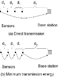
[image:3.612.404.505.236.368.2]

Cluster-head finally will create TDMA (Time Division Multiple Access) schedule for its associated members in the cluster.In Steady state phase starts when clusters have been created. In this phase nodes communicate to cluster-head during allocated time slots otherwise nodes completely keep sleeping. Due to this main attribute LEACH minimize energy dissipation and extend battery life of all individual nodes.

Figure 1. Direct transmission and Minimum transmission energy.

An amount of energy can be used in figure (a) is





2

2 1

3 d

d

K

amp





Whereas the amount of energy used in figure (b) is



2



2 2 1

3 d

d

K

amp





These are all the amount of energy depletion by data transfer formula.

Energy being dissipated to run the transmitter is

bit

nj

E

elec



50 /

.

Energy dissipation of the transmission amplifier is



_amp



100 pj

/

bit

/

m

2

.

Transmission cost is





_



Kd

K

E

d

K

E

_Tx

,



_elec



_amp

And finally the Receiving cost is

E

_Rx

 

K



E

_elec

K

Where

(4)

International Journal of Emerging Technology and Advanced Engineering

[image:4.612.80.253.427.596.2]

376

Figure 2. LEACH bad and good Scenario

Both of these diagrams is the optimum scenario, comparatively second is better because the cluster-heads are spaced out and the network is more properly sectioned in figure2.

In [3], new cluster head selection algorithm is established, in which cluster head is decided by Sink node according to its energy in the list. The main energy consumption of these handlings comes to sink node whose energy is free, therefore, ELEACH-M an balance energy consumption and prolong entire network period comparing with LEACH.

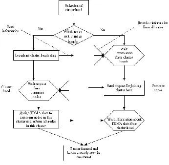
However, in ELEACH-M, cluster nodes frequently need to send control frame to cluster head, making waste energy of the network. Besides, the improvement of ELEACH-M a data delivery mechanism is only considered on the aspect of energy-efficiency, not data-efficiency. In [4] Zhou designs based on the Differentiated Services, which divides data into common and exigent. When dealing with common data, the request of data reliability is not very high, therefore, source node can choose a path to sink node depending on probability for data delivery, which can save energy. Emergency takes place only to ensure the exigent data delivered to sink is accurate, the source node will synchronously start all non-inter secant paths to Sink, satisfying users require for unexpected emergent events. In other words, this paper uses redundancy manner to improve its reliability. The following figure 4. Shows that different processes of nodes in LEACH protocol.

3.2 ELEACH-M (Enhancement of Multi-hop -

PROTOCOL)

(5)

International Journal of Emerging Technology and Advanced Engineering

[image:5.612.111.228.139.293.2]

377

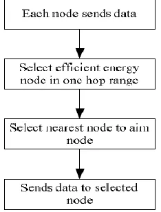
Figure 5. Routing of Enhancement of Multi-hop LEACH Protocol.

Authors in [7] introduced a new version of LEACH with a mobility factor. ELEACH-M uses the same threshold formula based on the original LEACH. It is used to calculate the threshold, but ELEACH-M takes into consideration the mobility of nodes during data transfer phase, which LEACH does not. The mobility itself is a challenge because mobile node can leave cluster while it is transmitting data to a CH. ELEACH-M solves this problem by confirming whether a mobile node still able to communicate with CH or not to TDMA schedule. In the beginning of each TDMA slot, the CHs transmit the message to REQ-DATA-TRANSMITION. If the mobile node is unable to receive the message then the CH waits for the request in the next TDMA slot and if the node misses two successive TDMA frames, it considers itself out of range, and the CH will remove unreachable nodes from its member list.

3.3 Analytical Model

We consider two models Model-1 &

Model -2, model -1 for single queue and model-2 for Double queue are shown in figures 6 & 7.

Fig 6. Model -1 Single queue

Figure 7. Model-2 .Double queue

We assume the following notions

λ1: Arrival rate of TCP Packets

λ2: Arrival rate of UDP Packets

μ1: service rate of TCP Packets

μ2: Service rate of UDP Packets

L: Length of queue

At: Number of TCP Packets arrived at queue

Au: Number of UDP packets arrived at queue

Pt: Number of TCP Packets stored at queue

Pu: Number of UDP packets stored at queue

Dt: Number of TCP Packets to be dropped in model-1

D’t:Number of TCP Packets to be dropped in model-2

Du : Number of UDP Packets to be dropped

Pdt: probability that dropping TCP packets in model-1

P’dt:probability that dropping TCP packets in model-2

Dt is computed as follows in model-1

D = [At-[L-(Pu+Pt) ] if [L-(Pu+Pt)] ≤ At

0 if [L-(Pu+Pt)] >At

Pdt is computed as follows

t t dt

A

D

P



D/t is computed in model -2 as follows

D’t = [At-(L / 2 - Pt)] if (L / 2- Pt) ≤ At

(6)

International Journal of Emerging Technology and Advanced Engineering

378 P/dt iscomputed as follows

t t dt

A

D

P

'



P’dt ≤ Pdt if ( Pu > L / 2)

Here we proved that Probability that dropping TCP packets in Model-2 is less than Probability that dropping TCP packets in Model-1.

IV. GAME THEORY

In early 1950's John Nash recognized that in non cooperative games there exist sets of optimal strategies (so-called Nash equilibrium) used by the players in a game such that no player can benefit by unilaterally changing his or her strategy if the strategies of the other players remain unchanged. Recently game theory has been used extensively to model networking problems, where different players may have different strategies for network usage. Game theory is a formal way to analyze interaction among a group of rational players who behave strategically. A game is the interactive situation, specified by the set of players (i.e., sensor nodes), the possible actions of each node, and the set of all possible payoffs. Games in which the actions of the players are directed to maximize their own profit without subsequent subdivision of the profit among the players are called Cooperative Games. Game theory provides a good framework with concepts of a coalition and coalitional value and different notions of stability.

Cooperative game-theoretic models can be used to do this for self-motivated agents (sensor nodes), each of which has tasks it must fulfill and resources it needs to complete these tasks. Although the agents (sensor nodes) can act and reach goals by themselves, it may be beneficial to join together. Behavior of sensor nodes can be coordinated based on Nash Equilibrium proposed in Game theory to achieve some desired objectives. The proposed game is

expressed as:

N

,

  

S

_i

,

P

_i where N is the set of sensor nodes, Si the set of strategies of sensor nodes, and Pi the

payoff function for node i.

(i) Payoff function

The payoff function between sensor nodes is composed of two important factors: cooperation, reputation. The Stronger cooperation between two nodes means the more reliable data communication between them. Also, the more a node cooperates, the better its reputation is.

The payoff between two sensor nodes should be dependent on their distance and each node's transmitter signal strength.

(ii) Game Strategy

Each sensor node utilize its strategy according to the information it attained in preceding time slots in the light of the following factor: (1) reputation



_ij sensor nodes have

not made enough reputation to trust each other and

cooperate with each other, (2) distance

d

_ij is the closer to

two nodes, the more they trust each other. All the sensor nodes will cooperate with each other successfully according to reputation level, and closeness of sensor nodes.

V. BAYESIAN THEORY OF GAMES

Bayesian rational prior equilibrium requires agent to make rational decisions and statistical predictions. Starting with first order non informative prior and keeps updating with statistical decision theoretic and game theoretic reasoning until a convergence of conjectures is achieved. So far we have been assuming that everything in the game was common knowledge for everybody playing, in fact the players may have private information about their own payoffs, about their type or preferences etc. In this situation the way of modeling of asymmetric or incomplete information is by recurring to an idea generated by Harsanyi (1967). The key is to introduce a move by the Nature, which transforms the uncertainty by converting an incomplete information problem into an imperfect information problem.

In a Bayesian game, a state refers to a possible scenario that may be realized in the game. Bayesian games are in multiple states and types that are used to summarize the degree to which each player can differentiate between the states. Due to instance, in a Bayesian game with two states, a player with two types can distinguish between the states while a player with one type cannot. For a player with multiple types in Bayesian, each type has a separate set of preferences that correspond with a particular state of the game. The idea is the Nature moves determining players’ types, a concept that embodies all the relevant private information about them such as payoffs, preferences, beliefs about other players, etc.

Definition 5.1:

(7)

International Journal of Emerging Technology and Advanced Engineering

379 (i) Players

i





1 ,

2 ,...

..

I



.

(ii) a finite action set for each player

a

_i



A

_i

(iii) A finite type set for each player



_i



ϴi

(iv) A probability distribution over type

p

/



(Common prior beliefs about the players’ types).

(v)Utilities





I I

i

A

XA

X

A

X

u

:

₁ ₂

...



₁



₂

...



Now it is important to discuss a little bit each part of the definition. Players’ types contain all relevant information about certain player’s private characteristics. The type



_i is only observed by player i , who uses this information both to make decisions and to update his beliefs about the likelihood of opponents’ type. (Using the conditional probability

p





__i

/



_i



. Combining actions and types for each player it’s possible to construct the strategies. Strategies will be given by a mapping from the type space

to the action space,

s

_i

:



_i



A

_I with elements

s

_i

 



_i . In words a strategy may assign different actions to different types. Finally, utilities are calculated by each player by taking expectations over types using his or her own conditional beliefs about opponents’ types. Hence, if player

i uses the pure strategy

s

_i, other players use the strategies

i

s

_ and player i‘s type is



_i, the expected utility can be written as



i i i





u

s

E

i

/

,



 



i i i i i

 

i i



i

s

p

u

i i



 

/

,

_ _ _ _







.

Bayesian Nash Equilibrium (BNE)

A Bayesian Nash Equilibrium is basically the same concept than Nash equilibrium with the addition that players need to take expectations over opponents’ types.

Definition 5.2:

A Bayesian Nash Equilibrium (BNE) is a Nash Equilibrium of a Bayesian Game, (i.e)



i i i



u



i i i



u

s

E

s

E

i

/

,



/

,



'





for all

s

i

 



i



S

i

'

and

for all types



_i occurring with positive probability.

Theorem 5.1: Every finite Bayesian Game has a Bayesian Nash Equilibrium.

VI. BAYESIAN NETWORK

The primary hypothesis variable for the Bayesian network was the degree of interest. We could not test the accuracy of prediction directly related to the hypothesis variable. Bayesian network survey includes two indicators of degree of interest, interpersonal counterproductive behavior and organizational counterproductive behavior. We used these variables as criteria to examine the extent to which the changes in the Bayesian network affected its ability to predict counterproductive behavior.

The following strategy was used to test the predictions of the Bayesian network. The network processed a number of cases in which the values of variables included in the paper. These values were entered into the network as findings (or evidence), and the network then predicted the probability of counterproductive behavior based on this evidence. The predicted values were then compared to the actual values to assess the correctness of the predictions. For the original and then the revised Bayesian network, we conducted this analysis for a set of cases simulated using the Bayesian network to get an upper bound on the possible accuracy of model prediction and repeated the analysis using actual cases from the survey data set. The two sources are (i) simulated cases that were generated by the Bayesian network itself, and (ii) empirical cases based on responses to the survey. The empirical cases were drawn directly from the survey measures, but were normalized to have means and standard deviations that corresponded to the comparable variables in the Bayesian network. The simulated cases provided a baseline against which the quality of the predictions of empirical cases was assessed.

VII. SIMULATION AND RESULTS

(8)

International Journal of Emerging Technology and Advanced Engineering

[image:8.612.54.283.159.646.2]

380

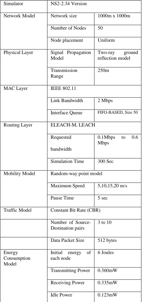
Table 1: Simulation Parameter

Simulator NS2-2.34 Version

Network Model Network size 1000m x 1000m

Number of Nodes 50

Node placement Uniform

Physical Layer Signal Propagation Model

Two-ray ground reflection model

Transmission Range

250m

MAC Layer IEEE 802.11

Link Bandwidth 2 Mbps

Interface Queue FIFO-BASED, Size 50

Routing Layer ELEACH-M, LEACH

Requested

bandwidth

0.1Mbps to 0.6 Mbps

Simulation Time 300 Sec

Mobility Model Random-way point model

Maximum Speed 5,10,15,20 m/s

Pause Time 5 sec

Traffic Model Constant Bit Rate (CBR)

Number of Source-Destination pairs

3 to 10

Data Packet Size 512 bytes

Energy Consumption Model

Initial energy of each node

6 Joules

Transmitting Power 0.360mW

Receiving Power 0.335mW

Idle Power 0.123mW

The ELEACH-M has been implemented by using Network Simulation-2(NS-2), it is a standard simulator. The channel bandwidth is 2 Mbps. A free space radio propagation model is used in which the signal power attenuates is 1/r2, where r is the distance between the nodes. All the nodes have the same transmission range of 250 meters. The distributed coordination function of IEEE802.11 is used MAC layer. All nodes can overhear packets destined for others. The nodes are deployed at random locations in a 1000mx 1000m region.

For the mobile scenarios, the random waypoint model is used for node mobility. In this model, a node chooses a random point in the network. It moves towards its destination point at a constant speed. The speeds are uniformly chosen between the minimum and maximum speeds and are set 0 m/s and 20 m/s, respectively. If the node reaches its destination point, it stays there for a certain pause time, after which it chooses another random destination point and repeats this process and the simulation ends after 300sec. The data traffic is generated by Constant Bit Rate (CBR) sessions initiated between the source and destination. All the nodes are assumed to have the same amount of battery capacity with full energy at the beginning of the simulation and initial energy of each node is 6 Joules. While transmitting power and receiving power of each node is 0.360mW and 0.335mW respectively. In this simulation, a group of data rates ranging from 32 kbps to 1024 kbps is applied, the mobility scenario is with a pause time of 3 seconds and the maximum node speed is 5 m/s.

The following quantitative metrics are used to measure the performance of protocols.

7.1 Packet Delivery Ratio

Packet Delivery Fraction (PDF):The ratio of the number of packets generated by the sources to the number of packets received by the destinations.

(9)

International Journal of Emerging Technology and Advanced Engineering

[image:9.612.59.274.108.670.2]

381

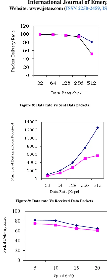
Figure 8: Data rate Vs Sent Data packets

Figure.9: Data rate Vs Received Data Packets

Figure.10: Data packet delivery ratio versus speed

From figure 8, it can be seen clearly that the LEACH-M and ELEACH-M have approximately equal PDR at low data rate (data rate below 512 kbps). When the data rate of traffic flow increases to kbps to 256 kbps. The PDR of LEACH suddenly drops from 98% to 60%. At higher data rates ELEACH-M performs better than to LEACH, because In the ELEACH-M, the route is selected based on bandwidth and energy. Packet delivery ratio is directly proportional to the bandwidth and energy. Fig.9 shows that number received data packets in ELEACH-M are greater than number received data packets in LEACH.

The comparison of packet delivery rate Vs speed is shown in figure 10. The packet delivery rate of ELEACH-M is higher than LEACH due to less link breaks. In LEACH, three events may occur; solution is immediately alternative path is chosen without delay. The probability of link failure in the ELEACH-M is less than the probability of link failure in the LEACH, as the speed of the nodes increases, the probability of link failure increases and hence the number of packet drops also increases. The ELEACH-M has higher packet delivery ratio than LEACH.

7.2 End -To-End Delay

Average end-to-end delay is the delay of data propagation, transfer and the delays caused by queuing, buffering and retransmitting data packets. The delay of each packet= the time of received data packets - the time of sent this data packet. The average end to end delay is then computed as: Average delay =Total delay of each data packets / total data packets received.

(10)

International Journal of Emerging Technology and Advanced Engineering

382

0 0.5 1 1.5 2 2.5 3 3.5 4

32 64 128 256 512

A

ve

ra

ge

De

la

y (m

s)

[image:10.612.60.284.137.417.2]

Data Rate (Kbps)

Figure 11: Data rate Vs Average Delay

Figure 12. Average delay Vs Speed

From figure 11, it can be seen clearly that the ELEACH-M and LEACH have low and approximately equal average delay at low data rate (data rate below 256 kbps). When the data rate of traffic flow increases to kbps to 512 kbps. It shows that networks with the ELEACH-M routing protocol can provide lower end to end delay for traffic flows than the LEACH because the ELEACH-M always choose to find a route with satisfying data rate and energy. In addition to that, during the transmission, the QoS of the traffic is monitored.

Figure 12 depicts the variation of the average end-to-end delay as a function of mobility of nodes. It can be seen that the general trend of all curves is an increase in delay with the increase of velocity of nodes. Mainly the reason is that high mobility of nodes results in an increased probability of link failure that causes an increase in the number of routing rediscovery processes. This makes data packets have to wait for more time in its queue until a new routing path is found.

The delay of ELEACH-M remains approximately equal at all Static sinks. In LEACH, the delay increases quickly as node mobility increases. In the availability of alternate node-disjoint routing paths in ELEACH-M eliminates route discovery latency that contributes.

In addition, when a congestion state occurs in a routing path, the source node is distributed incoming data packets to the other node-disjoint routing paths to avoid the congestion. This reduces the waiting time of data packets in queue.

7.3 Routing Overhead

It is equal to the number of routing packets transmitted per data packet delivered at destination. Each hop-wise transmission of a routing packet is counted as one transmission. It is also known as Normalized Routing Load (NRL). It is also defined as NRL =Number of control packets generated /number of received data packets

The routing overhead is an important metric to compare the performance of different protocols since it gives a measure of the efficiency of protocols, especially in a low bandwidth with congested wireless environments. Protocols that transmit a large number of packets can also increase the probability of packet collisions and waiting time of data packets in transmission buffer queues.

0 1 2 3 4 5 6 7 8 9

32 64 128 256 512

Ove

rh

ea

d

[image:10.612.347.523.365.684.2]

Data Rate (Kbps)

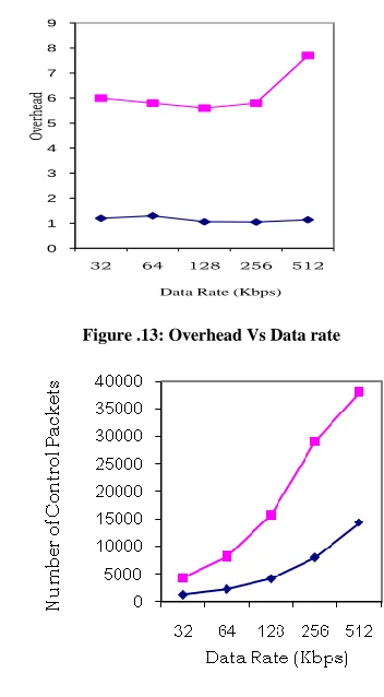
Figure .13: Overhead Vs Data rate

[image:10.612.360.502.374.501.2]

(11)

International Journal of Emerging Technology and Advanced Engineering

383

0 20 40 60 80 100 120 140 160 180

5 10 15 20

N

umb

er

o

f

C

on

tr

ol

P

ac

ke

ts

[image:11.612.71.273.145.253.2]

Speed(m/s)

Figure 15: Number of control packets Vs Speed

Figure 13 shows the Overhead Vs data rate. At low mobility; single path routing generates less overhead than multipath. At high mobility, frequently links failure, so the route discovery is repeatedly performed by the sources to find new routes due to overhead increases. It has shown that the normalized routing load in ELEACH-M performs better than the LEACH when speed increases. The normalized routing load in LEACH increases more quickly than that in ELEACH-M with the increase of mobility. ELEACH-M generates less overhead due the following reason, while during route discovery itself. It eliminate the some paths if they don’t support QoS, this result in an increased packet delivery ratio, decreasing end-to-end delays for data packets, lower control overhead, and fewer collisions of packets . Figure 14 and fig.15 show the number of control packets Vs date and the number of control packets and speed respectively

7.4 Energy consumption

The nodes in a WSN are typically powered by batteries which have limited energy reservoir. It becomes very difficult to recharge or replace the battery of nodes. In such situations energy conservations are essential. The lifetime of the nodes show strong dependence on the lifetime of the batteries. In the WSN nodes depend on each other to relay packets and the list of some nodes may cause significant topological changes, undermine the network operation, and affect the lifetime of the network.

[image:11.612.345.522.148.316.2]

The comparison of energy consumption is shown Fig.16 and fig 17.

Figure 16. Energy consumption against Data rate

0 0.5 1 1.5 2 2.5

0 5 10 15 20

En

erg

y

C

on

s

um

pt

io

n

(

J

ou

le

s

)

Life Time(m/s)

LEACH ELEACH-M

Figure 17. Energy consumption against Lifetime

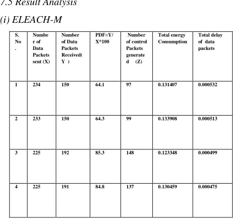
7.5 Result Analysis

(i) ELEACH-M

S. No .

Numbe r of Data Packets sent (X)

Number of Data Packets Received( Y )

PDF=Y/ X*100

Number of control Packets generate d (Z)

Total energy Consumption

Total delay of data packets

1 234 150 64.1 97 0.131407 0.000532

2 233 150 64.3 99 0.133908 0.000513

3 225 192 85.3 148 0.123348 0.000499

[image:11.612.324.555.506.723.2]

(12)

International Journal of Emerging Technology and Advanced Engineering

384 (ii) LEACH

S . N o

Number of Data Packets sent X

Number of Data Packets Received Y

PDF =Y/X *100

Number of control Packets generate d Z

Total energy Consumption

Total delay of data packets

1 83 53 63.8 99 0.330219 0.003268

2 83 53 63.8 101 0.340238 0.003287

3 81 60 74 149 0.327602 0.002311

4 80 62 77.5 139 0.336445 0.002097

VIII. CONCLUSION

In this paper, we proposed an energy efficient protocol for WSNs. Our approach can be useful for applications that require scalability, prolonged network lifetime and node are dispersed in a large spacious field. It depends on overhead and load, the path failure mainly depends on due to lack energy of any one node on selected path. That it was eliminated in ELEACH-M. The ELEACH-M consumes less energy than to LEACH and to maximize the lifetime of network. Each node maintains minimum energy level dring the transmission of data, each node checks whether its energy reaches to threshold or not. If its energy reaches to threshold value, then node sends a EERP packet to the source node in reverse path. The source node immediately selects the alternate route.

REFERENCES

[1] Akyildiz and W. Su, Y. Sankarasubramaniam and E. Cayirci, “A Survey on Sensor Networks”, IEEE Commun. Mag., vol. 8, (2002), pp. 102.

[2] WANG Xuan-zheng, LI La-yuan, ZHANG Wei-hua, and ZHANG Liu- min, “Research on routing protocol for wireless sensor networks”, APPLICATION RESEARCH OF COMPUTERS, 2009, pp. 26(4). 1453–1455.

[3] Zhou Xin-Lian, Wang Run-Yun, “Reliable Data Delivery Algorithm based on Differentiated Service in WSNs”, Electronic Computer Technology, 2009 International Conference on 20-22 Feb. 2009 pp. 596–599.

[4] W. Heinzelman, A. Chandrakasan, and H. Balakrishnan, ”Energy-efﬁcient routing protocols for wireless microsensor networks,” in Proc. 33rdHawaii Int. Conf. SystemSciences(HICSS), Maui, HI,Jan. 2000.

[5] Heinzelman W. B., Chandrakasan A. P., Balakrishnan H., ”An application- speciﬁc protocol architecture for wireless microsensor networks,” IEEE Trans on Wireless Communications, Vol. 1, No. 4, 2002, pp. 660-670, doi: 10.1109/TWC.2002.804190.

[6] X. H. Wu, S. Wang, ”Performance comparison of LEACH and LEACH- C protocols by NS2,” Proceedings of 9th International Symposium on Distributed Computing and Applications to Business, Engineering and Science. Hong Kong, China, pp. 254-258, 2010 [7] P.T.V.Bhuvaneswari and V.Vaidehi ”Enhancement techniques

incorpo- rated in LEACH- a survey”Department of Electronics Engineering, Madras Institute Technology, Anna University Chennai, India, 2009.

[8] D. S. Kim and Y. J. Chung, "Self-organization routing protocol supporting mobile nodes for wireless sensor network," in Proc. First International Multi-Symposiums on Computer and Computational Sciences, Hangzhou, China, 2006.

[9] C. Xu and L. Cao, G. A. Zhang and J. Y. Gu, Editors, “Application Research of Computers”, vol. 3, (2010), pp. 816.

[10] W. Heinzelman, A. Chandrakasan and H. Balakrishnan, “Energy-efficient Routing Protocols for Wireless Microsensor Networks”, Proceedings of the 33rd Annual Hawaii International Conference of System Sciences, (2000) January 4-7; Maui, Hawaii.

[11] S. Lindsey and C. S. Raghavendra, Editors, “PEGASIS: Power-efficient Gathering in Sensor Information Systems”, Parallel and Distributed Systems, vol. 9, (2002), pp. 924.

[12] O. Younis and S. Fahmy, Editors, “HEED: A Hybrid, Energy-efficient, Distributed Clustering Approach for Ad Hoc Sensor Networks”, Mobile Comput., vol. 3, (2004), pp. 366.

[13] B. S. Lee, H. W. Lin and W. Tarng, “A Cluster Allocation and Routing Algorithm Based on Node Density for Extending the Lifetime of Wireless Sensor Networks”, Proceedings of the 26th International Conference on Advanced Information Networking and Applications Workshops (WAINA), (2012) March 26-29; Fukuoka, Japan.

[14] Y. Hu and X. R. Shen and Z. H. Kang, “Energy-efficient Cluster Head Selection in Clustering Routing for Wireless Sensor Networks”, Proceedings of the 5th International Conference on Wireless Communications, Networking and Mobile Computing (2009) September 24-26; Beijing, China.

[15] X. X. Zhang and M. Zhang, Z. C. Zhang, “An Improved WSNs Clustering Routing Algorithm and Its Performance”, Science paper Online, vol. 2, (2010), pp. 96.

[16] M. C. M. Thein and T. Thein, “An Energy Efficient Cluster-head Selection for Wireless Sensor Networks”, Proceedings of International Conference on Intelligent Systems, Modelling and Simulation (ISMS), (2010) January 27-29; Liverpool, United Kingdom.

[17] J. F. Qiao, S. Y. Liu and X. Y. Cao, “Density-based Clustering Protocol for Wireless Sensor Networks”, Computer Science, vol. 12, (2009), pp. 46.

[18] A. Schillings and K. Yang, “VGTR: A Collaborative, Energy and Information Aware Routing Algorithm for Wireless Sensor Networks Through the Use of Game Theory”, Lecture Notes in Computer Science, vol. 5659, (2009), pp. 51.

[19] B. Arisian and K. Eshghi, “A game theory approach for optimal routing in wireless sensor networks”, Proceedings of the 6th International Conference on Wireless Communications Networking and Mobile Computing (WiCOM), (2010) September 23-25; Chengdu, China.

(13)

International Journal of Emerging Technology and Advanced Engineering

385 [21] J. Hu and L. F. Shen, “Clustering Routing Protocol of Wireless

Sensor Networks Based on Game Theory”, Jornal of Southeast Uniwersity, vol. 3, (2010), pp. 441.

[22] F. Kazemeyni, E. B. Johnsen and O. Owe, Editors, “Grouping Nodes in Wireless Sensor Networks Using Coalitional Game Theory”, Proceedings of the 16th IEEE International Conference on Engineering of Complex Computer Systems (ICECCS), (2011) April 27-29; Las Vegas, Nevada USA.

[23] G. Z. Zheng, S. Y. Liu and X. G. Qi, “Clustering Routing Algorithm of Wireless Sensor Networks Based on Bayesian Game”, Journal of Systems Engineering and Electronics, vol. 1, (2012), pp. 154.

[24] D. Lee, H. Shin and C. Lee, “Game theory-based resource allocation strategy for clustering based wireless sensor network”, Proceedings of the 6th International Conference on Ubiquitous Information Management and Communication (ICUIMC '12), (2012) February; Kuala Lumpur, Malaysia.

[25] T. Rappaport, Editor, “Wireless Communications: Principles & Practice”, Englewood Cliffs, Prentice-Hall (1996). [24] D. Fudenberg and J. Tirole, Editors, “Game Theory”, MIT Press, (1991).