462
ULTRASONIC TIME OF FLIGHT COMPUTED
TOMOGRAPHY FOR CONCRETE INSPECTION
1, 2
HONGHUI FAN, 1HONGJIN ZHU
1School of Computer Engineering, Jiangsu Teachers University of Technology, Changzhou, 213001, China
2Key Laboratory of Cloud Computing & Intelligent Information Processing of Changzhou City, Jiangsu
Teachers University of Technology, Changzhou, 213001, China
ABSTRACT
This research aims to evaluate the internal structure of concrete material configuration using an immersed ultrasonic computed tomography imaging technique. We propose a relative difference method of time of flight data to remove distortions in imaging process of concrete. Time of flight data for 306 paths were measured in total by manual scanning for one computer tomography image, we examined interpolation of time of flight data as the density which has a considerable effect on image quality in Filtered Back Projection (FPB) method. The relative difference of time of flight and interpolation is examined in detail using concrete phantoms. The accuracy of defect detection in concrete was significantly improved by the proposed technique.
Keywords: Ultrasonic Computed Tomography, Time Of Flight, Concrete, Reconstruction Image
1 INTRODUCTION
Ultrasonic computed tomography which has been used as the object’s internal-structure imaging technique is able to map the physical quantity distribution within the object non-destructively (non destructive testing). It is an alternative way for quality inspection of many materials. The ultrasonic wave for nondestructive testing of concrete was repeatedly identified as being of high priority. The application of this reconstruction concept is then employed by some experts, such as Bracewell to reconstruct images of microwave emission from the solar surface[1], Imoto et al. studied image reconstruction using low-frequency for ultrasonic testing of concrete[2].
The research on the application of computed tomography for quality inspection of concrete is being done, it will be very appropriate for regular testing and in situnondestructive testing during concrete construction exists. The ultrasonic wave for nondestructive testing of concrete was repeatedly identified as being of high priority. Currently, the content of concrete inspection is cracked and holes. He-Ning proposed geometric active contour model for concrete computed tomography image[3],Chai used attenuation of ultrasonic for concrete tomography reconstruction[4]. However, these methods cannot achieve the real internal structure
visualization. Ultrasonic time of flight use ultrasonic signal which through the interior of measured object to reconstruct ultrasonic images. At the ultrasonic time of flight computed tomography, the spatial distribution of sound velocity is estimated, so using ultrasonic time of flight we can get concrete structure images.
ISSN: 1992-8645 www.jatit.org E-ISSN: 1817-3195
463
2 IMAGING PROCESS
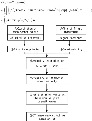
2.1 Image Reconstruction Using Fbp Algorithm The Filtered Back Projection algorithm uses Fourier theory to arrive at a closed form solution to the problem of finding the linear attenuation coefficient at various points in the cross-section of an object [11]. A fundamental result linking Fourier transforms to cross-sectional images of an object is the Fourier Slice Theorem [12, 13], in this paper we concerned only with parallel beam projection data. The Fourier Slice Theorem for the parallel beam projection data is given here. The same justifications
can be made for fan beam and cone beam projection data.
In the Equine (1) above, the terms inside the square brackets (the operation indicated by the inner integral) represents a filtering operation and evaluate the filtered projections. The operation being performed by the outer integral evaluate the back-projections, which basically represents a smearing of the filtered projections back onto the object and then finding the mean over all the angles. The process of reconstruction image based on FBP method in our system was shown in Figure 1.
(
)
(
)
(
)
(
)
cos , sin
( cos sin , sin cos exp 2
( , ) exp 2
F
f f r s r s ds j r dr
p r j r dr
ρ θ ρ θ
θ θ θ θ πρ
θ πρ
∞ ∞
−∞ −∞ ∞
−∞
⎡ ⎤
= ⎢ − + ⎥ −
⎣ ⎦
= −
∫ ∫
∫
(1)
①Coor di nat es of
measur ement poi nt s ②Ti me of f l i ght measur ement
Si gnal t r eat ment
④Sound vel oci t y ③Poi nt i nt er pol at i on
⑤Vel oci t y i nt er pol at i on Fr om 306 t o 2556
⑥r el at i ve di f f er ence of sound vel oci t y 36 poi nt ( 10° i nt er val )
⑦Rat i o of pi xel val ue t o t he number of pi xel
t r ansi t waves
⑧CT i mage r econst r uct i on based on FBP ①Coor di nat es of
measur ement poi nt s ②Ti me of f l i ght measur ement
Si gnal t r eat ment
④Sound vel oci t y ③Poi nt i nt er pol at i on
⑤Vel oci t y i nt er pol at i on Fr om 306 t o 2556
⑥r el at i ve di f f er ence of sound vel oci t y 36 poi nt ( 10° i nt er val )
⑦Rat i o of pi xel val ue t o t he number of pi xel
t r ansi t waves
[image:2.612.159.456.245.634.2]⑧CT i mage r econst r uct i on based on FBP
Figure 1: Flowchart For Reconstruction Image Based On FBP
2.2 Measurement And Materials
The materials which used in our system were produced by the Atati Laboratory and YastakaYanagida Laboratory of Yamagata University. All of the data used in this paper were
from the same experimental system which was explained by Yanagida et al[5].
464 imaging method" to reduce the artifacts of reconstruction images based on FBP method for wood CT image reconstruction. In our system, the CT image was reconstructed based on the assumption that an ultrasonic wave was transferred along the straight line. However, an ultrasonic wave in the interior of the object wave propagation. To consider the ultrasonic characteristics, the relative time of flight method was performed. According our measurement method, all ultrasonic time of flight data grouped with a gap angle θc of the transmitter and the receiver (measuring angles from 20 to 180 with 20 intervals).
The average sound velocity of the same gap
(gap)
ave
v was calculated using
35 ( ) ( ) 0 1 36 gap gap ave i i v v =
=
∑
(2)L was the length of measurement path, T was the
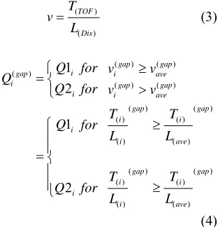
time of flight of with the same measurement path L. So the sound velocity of the measurement path was calculated using ( ) ( ) TOF Dis T v L
= (3)
( ) ( ) ( ) ( ) ( ) ( ) ( ) ( ) ( ) ( ) ( ) ( ) ( ) ( ) ( ) ( ) ( ) 1 2 1 2 gap gap i
gap i ave
i gap gap
i i ave
gap gap i i i i ave gap gap i i i i ave
Q for v v
Q
Q for v v
T T Q for L L T T Q for L L ≥ ⎧
= ⎨ >
⎩ ≥ ⎧ ⎪ ⎪ = ⎨ ⎪ ⎪ ≥ ⎩ (4)
The sound velocity (gap)
i
v must be almost the
same for one same gap pathways if the sample is normal (no defect). If (gap)
i
v was considerably
slower than the (gap)
ave
v (average velocity of the gap),
some defect should be on the i-th pathway. So
( ) ( )
1 gap gap
i th
Q =v was used for the clear pathway
instead of the time of flight value, and
( ) ( )
2 gap gap
i i
Q =v was used to for the defect in the
Equine (4).
Nine (gap)
i
Q groups after relative time of flight
method were used to reconstruct one CT image. As the influence of the anisotropic acoustic property was reduced, the artifact level of the reconstructed image decreased.
2.4 Interpolation
Measurement points were arranged at 10º intervals. It took about two hours to obtain 306 time of flight data from 20º intervals. So, the number of data that can be measured is thought that 306 were near the upper bound timely and spatially. The interval of measuring point and the number of time of flight path was determined by the size of specimens and the wavelength of ultrasonic. The interval of the measuring point should be smaller than the wavelength. So, start measuring from 20 º intervals, until end of the diameter of the measurement phantom. There was an exchange when transmitting and receiving on the same measurement point. Therefore, all the measurement paths should be 306 [= (transmitter 36 × receiver 18) /exchange 2- diameter 18], all measurement paths of one measurement point were shown in Figure 2(a). However, it is indicated that 306 data were not sufficient to obtain a clear CT image by the FBP method. Because of the lack of time of flight data, artifacts appeared in the FBP CT images [see Figure 3(b)].
To remove the artifact, angle interpolation was used in imaging process. Fan-beam was connected lines that arranged from the measurement point 0 to 35. When the intervals of transmitter and receiver were 10º intervals and 5º intervals, fan-beam of crossing paths would be made detailed. Because of all paths that could be calculated, so the interpolation data were increased. When the intervals of transmitter and the transducer were 5º intervals, 72
measurement points were assumed on the circumference of the test sample and labeled with numbers from 0 to 71. Figure 2(c) showed the paths and measurement points after interpolation. After
10 interpolation, the estimated time of flight data
[image:3.612.140.296.364.526.2]ISSN: 1992-8645 www.jatit.org E-ISSN: 1817-3195 465 0 9 18 27 0 18 27 9 0 18 36 54
20º intervals TOF 10º intervals TOF 5º intervals TOF 0 9 18 27 0 18 27 9 0 18 36 54 0 9 18 27 0 18 27 9 0 18 36 54
20º intervals TOF 10º intervals TOF 630
5º intervals TOF 2556 306
(a) (b) (c)
0 9 18 27 0 18 27 9 0 18 36 54
20º intervals TOF 10º intervals TOF 5º intervals TOF 0 9 18 27 0 18 27 9 0 18 36 54 0 9 18 27 0 18 27 9 0 18 36 54
20º intervals TOF 10º intervals TOF 630
5º intervals TOF 2556 306 0 9 18 27 0 18 27 9 0 18 36 54 0 9 18 27 0 18 27 9 0 18 36 54
20º intervals TOF 10º intervals TOF 5º intervals TOF 0 9 18 27 0 18 27 9 0 18 36 54 0 9 18 27 0 18 27 9 0 18 36 54
20º intervals TOF 10º intervals TOF 630
5º intervals TOF 2556 306
[image:4.612.88.513.73.246.2](a) (b) (c)
Figure 2: The Interpolation In The Case Of Fan Bean Geometry
3 RESULTS
3.1 Numerical Phantom
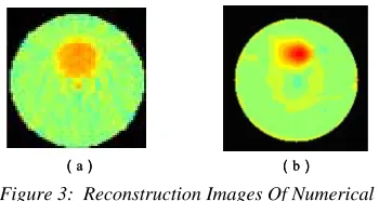
A numerical phantom containing a circle shaped defect was assumed which was composed of 128 x 128 square pixels of 1 mm size. The acoustic velocities were 5000 m/s for normal part, the acoustic velocities 2500 m/s for defect part. The diameter of specimen was 128. The defect was set of coordinates x=128, y=80, and radius r=15. The reconstruction images based on FBP method are shown in Figure 3.
(a) (b)
[image:4.612.111.286.421.514.2](a) (b)
Figure 3: Reconstruction Images Of Numerical Phantom
From the reconstructed images which without interpolation, some artifacts were observed in the images and no clear defects were observed. The number of time of flight data after 5º intervals interpolation was 2556. When time of flight interpolation was used, better-quality images could be obtained. In our simulation, we did not consider the undulatory property. Furthermore, the time of flight data from the numerical phantom did not take into account the effect on the anisotropic acoustic property.
3.2 Cconcrete Phantom
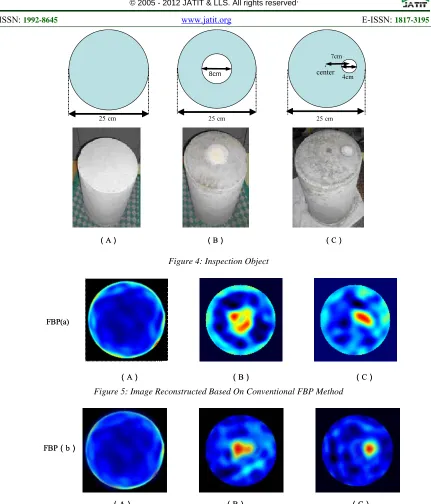
Three pieces of concrete phantom were prepared as test specimens. The materials of test specimens were mortar and polystyrene foam. Test specimen (a) was no defect. Test specimen(b) had a defect
which was set in the center, and the diameter was 8cm. Test specimen(c) had a defect which was set from the center 7cm, and the diameter was 4cm. All of the test specimen diameters were 25cm.
The images in Figure 5 were reconstructed by the conventional FBP(a) method with interpolation time of flight data. In the FBP (b) method, the relative difference method of time of flight was taken into account before interpolation. The CT images were successfully reconstructed based on FBP(a) method. The defect position of (B) specimen and (C) specimen were observed, but, it was possible that some artifacts were recognized in Figure 5. It was difficult to accurately judge the position of the defect. The anisotropic acoustic property was considered in the reconstructed images by the FBP(b) method in Figure 6, in which the number of line artifacts was reduced considerably and the artifacts on the edge of the reconstructed images almost disappeared. We could clearly find the defect in the reconstructed images of Figure 5.
4 CONCLUSIONS
466
25 cm
8cm
25 cm
4cm 7cm
●
center
25 cm
(A) (B) (C)
(A) (B) (C)
Figure 4: Inspection Object
(A) (B) (C)
FBP(a)
(A) (B) (C)
[image:5.612.92.523.64.568.2]FBP(a)
Figure 5: Image Reconstructed Based On Conventional FBP Method
(A) (B) (C)
FBP(b)
(A) (B) (C)
FBP(b)
Figure 6: Image Reconstructed Considered Relative Difference Method Of Time Of Flight
ACKNOWLEDGEMENTS
The authors are very thankful to Atati Laboratory and Yanagida Laboratory from Yamagata University of Japan for providing experimental data. This work was supported by the Foundation of Jiangsu Teachers University of Technology (KYY11049 and KYY11048) and the Key Laboratory of Cloud Computing & Intelligent Information Processing of Changzhou City (No. CM20123004.).
REFRENCES:
[1] Bracewell R.N and Wernecke S.J, “Image reconstruction over a finite field of view”, Journal of the Optical Society of America, Vol. 65, No. 11, pp. 1342-1346.
ISSN: 1992-8645 www.jatit.org E-ISSN: 1817-3195
467 [3] HE Ning, LU Ke, and BAO Hong, “An
Improved Geometric Active Contour Model for Concrete CT Image Segmentation Based on Edge Flow”, Chinese Journal of Electronics, Vol. 16, No. 4, pp. 697-690.
[4] H.K. Chai, S. Momoki, Y. Kobayshi et al, “Tomographic reconstruction for concrete using attenuation of ultrasound”, NDT & E International, Vol. 44, No. 2, pp. 206-215. [5] H. Yanagida, Y. Tamura, KM. Kim et al,
“Japanese Journal of Applied Physics”, Vol. 46, pp. 5321-5325.
[6] KM. Kim, JJ. Lee, SJ. Lee, et al, “Wood and Fiber Science”, Vol. 40, No. 4, pp. 572-579. [7] Honghui Fan, Shuqiang Guo, Y. Tamura et al, “
Time of flight ultrasonic CT based on ML-EM for wooden pillars”, Ultrasonic Symposium in Bejing, IEEE Conference Publishing Services, November 2-5, 2008, pp. 1495-1498.
[8] S. Kusminarto, G. Bayu, and A. Sugiharto, “International Journal of Civil & Environmental Engineering”, Vol. 11, No. 5, pp. 17-22. [9] Honghui Fan, Hongjin Zhu, Guangping Zhu et
al, “Improvement of Wood Ultrasonic CT Images by Using Time of Flight Data Normalization”, Vol. 6, No. 6, pp. 1079-1083. [10] Honghui Fan, H. Yanagida, Y. Tamura et al,
“Japanese Journal of Applied Physics”, Vol. 49, pp. 07HC12 (6 pages).
[11] F. Natterer, “Mathematics for computer tomograhpy”, 1996, pp. 180-212.
[12] F. M. Dickey, A. W. Doerry, “Recovering shape from shadows in synthetic aperture radar imagery”, Proceeding of SPIE on Radar Sensor Technology XII, May 13, 2008, pp. 694707 (12 pages).