SOLVING ECONOMIC DISPATCH PROBLEM USING PARTICLE SWARM OPTIMIZATION BY AN EVOLUTIONARY TECHNIQUE FOR INITIALIZING PARTICLES

966

TWO-LEVEL STRUCTURE FOR ANALOG CIRCUIT FAULT

DIAGNOSIS USING IMPROVED DAGSVM AS CLASSIFIER

KE GUO,YI ZHU,YE SAN

School of Astronautics, Harbin Institute of Technology, Harbin 150001, Heilongjiang, China

ABSTRACT

Fault diagnosis of analog circuit is of essential importance for guaranteeing the reliability and maintainability of electronic systems. Taking into account the requirements and characteristics of analog circuit fault diagnosis, two-level diagnostic structure for analog circuit is proposed in this paper. Analog circuit fault diagnosis can be regarded as a pattern recognition issue and addressed by multi-class SVM. Aiming at the uncertainty of the node arrangement and the error accumulation phenomenon, the improved directed acyclic graph support vector machine (DAGSVM) based on fisher separability measure in high dimensional feature space and margin of SVM is proposed. In order to eliminate redundant fault features and the impact of measure noise on the diagnostic accuracy, simultaneously taking into account lightening the workload of the classifier, the separability promotion algorithm based on kernel principal component analysis (KPCA) plus linear discriminant analysis (LDA) is proposed. Then the separability promotion algorithm is used to extract the nonlinear fault features of analog circuit and the two-level structure based on improved DAGSVM is applied to diagnose faults in analog circuit. The unbalanced classification model based on SVM is adopted in the first level. The effectiveness of the proposed method is verified by the experimental results.

Keywords: Fault Diagnosis, Analog Circuit, Improved DAGSVM, Separability Promotion Algorithm, Kernel Principal Component Analysis

1. INTRODUCTION

The normal operations of aircraft are guaranteed by the reliable avionic equipment to a considerable extent. With the integration and the increasing scale of electronic devices, the reliability and research of avionics equipment are of great significance [1]. Generally speaking, the circuit system of avionic equipment can be divided into digital circuit and analog circuit. Above 80% of the circuits in electronic equipment is digital, but virtually 80% of the faults occur in analog circuits [2, 3]. Fault diagnosis of digital circuit has reached the point of automation, while that of analog circuits is still challenging due to component tolerances, circuit nonlinearities measurement noise and poor fault models [4]. These difficulties make the application of artificial intelligence techniques to these problems very attractive. Analog circuit fault diagnosis can be regarded as a pattern recognition issue and addressed by artificial neural network or support vector machine. Neural Network has excellent classification capability and self-learning ability, and can approximate any nonlinear function in theory when the number of hidden layer nodes is sufficient.

ISSN: 1992-8645 www.jatit.org E-ISSN: 1817-3195

967 circuit in recent years [9-11]. In literature [9], a novel analog circuit fault diagnosis approach based on improved one-against-rest SVM is proposed, but the drawback of the approach is that the number of the required accessible nodes is up to 6. In literature [10], a new approach of fault diagnosis in analog circuits, which employs the fractional wavelet transform to extract fault features and adopts a fuzzy multi-classifier based on the support vector data description to diagnose circuit faults, is proposed. A threshold value is adopted to decrease the fuzzy region which in the overlap between hyperspheres, but it is difficult to select a reasonable threshold.

An improved directed acyclic graph SVM method is proposed and then adopted to diagnose analog circuit faults in this paper. Taking into account the importance of preprocessing the output data of the circuit under test, kernel principal component analysis (KPCA) plus linear discriminant analysis (LDA) is adopted as a preprocessor. The paper is organized as follows. In section 2, the principle and implementation steps of separability promotion algorithm based on kernel principal component analysis and linear discriminant analysis are given. In section 3, the improved DAGSVM is given. This is followed by two-level structure for analog circuit fault diagnosis and the exper-imental results. Finally, conclusions are given in section 5.

2. SEPARABILITY PROMOTION

ALGORITHM BASED ON KPCA PLUS LDA

KPCA is first developed by Schölkopf [12] based on the theory of reproducing kernel Hilbert space. Due to better performance of nonlinear features extraction and noise elimination as compared with PCA, KPCA has gained substantial attention as a learning machine in pattern recognition, statistical analysis and image processing. The features extracted by KPCA are not optimal classification features but optimal description features. In order to solve the problem, a novel approach of data reconstruction by KPCA and processed by LDA which named separability promotion algorithm is proposed.

2.1Kernel Principal Component Analysis

Consistent with Cover’s theorem, it has been shown that nonlinearly separable patterns in the original input space may be transformed such that they are linearly separable in a high dimensional space via a nonlinear mapping. This high

dimensional linear space is referred to as the feature spaceF . The basic idea of KPCA is to map the input data m

x∈R into a new high dimensional feature spaceF firstly via a nonlinear mapping

( )

φ ⋅ , and then perform a linear PCA inF .

Let X =[ ,x x_{1 2},,x_n]( ∈ m i

x R ,i=1, 2,,n) be the observation set, where n is the sample number,

m is the number of variables. By the nonlinear mappingφ: φ( )∈ h

x x F , the measured inputs are extended into the high dimensional feature space, where his the dimension in feature space which is assumed to be a sufficiently large number. The sample covariance matrix in the feature space can be expressed by

1 1

( ( ) )( ( ) )

φ φ φ φ φ

=

=

∑

n − − T

i i

i

C x m x m

n (1)

where

1 1

( )

φ φ

=

=

∑

n _i

i

m x

n is the sample mean. We

denote φ( )x_i =φ( )x_i −m_φ as the centered feature space sample.

Then formula (1) can be expressed as

1 1

( ) ( )

φ φ φ

=

=

∑

n T

i i

i

C x x

n (2)

For convenience, we assume that φ( )xi have

been centralized, where i=1, 2,n.

The kernel principal component can be obtained by solving the eigenvalue problem in the feature space:

1 1

( ( ), ) ( ) φ

λ φ φ

=

= =

∑

n T

i i

i

v C v x v x

n (3)

where eigenvalues λ ≥0and eigenvectors v∈F .

It is easy to see that every eigenvector vof Cφ

lies in the span of φ( ),x1 , (φ xn). Hence λ =v C vφ

is equivalent to

( ( ), ) ( ( ), _φ )

λ φ x_k v = φ x_k C v (4)

where k=1, 2,,nand there exist coefficients α_i, 1, 2, ,

= 

i n. Such that

1

( )

α φ =

=

∑

n _{i i} i

v x (5)

968 1

1 1

( ( ), ( ))

1

( ( ), ( ))( ( ), ( ))

λ α φ φ

α φ φ φ φ

=

= =

=

∑

∑

∑

n

i k i

i

n n

i k j j i

i j

x x

x x x x

n

(6)

Defining kernel matrix K with size n n× by [ ]K ij =( ( ), (φ xi φ xj)) , then its elements are determined by virtue of kernel tricks.

[ ]K _ij =( ( ), (φ x_i φ x_j))=κ( ,x x_{i j}) (7)

where κ( ,x x_{i j}) is the calculation of the inner product of two vectors in feature spaceF with a kernel function. This reads

2

λ α= α

n K K (8)

whereα denotes the column vector with entries

1, 2, ,

α α  α_n. To get solutions of equation (8), we solve the eigenvalue problem, and it is equivalent to perform PCA inF .

λα= α

n K (9)

Let λ₁≥λ₂≥≥λ_n denote the eigenvalues of

K , and α α1, 2,,αn the corresponding complete

set of eigenvectors. The dimensionality of the problem can be reduced by retaining only the first

p eigenvectors. We normalize α α1, 2,,αp by

requiring that the corresponding vectors in feature space F be normalized, i.e., ( ,v vk k)=1 for all

1, 2, ,

= 

k p. According to equation (5) we get

1 1

( α φ( ), α φ( )) 1

= =

=

∑

n

∑

n

k k

i i j j

i j

x x (10)

Further, we get

1 1

( α φ( ), α φ( )) λ α α( , )

= =

==

∑

n

∑

n

k k

i i j j k k k

i j

x x (11)

Knowing the normalized vectors , the PCs t of a test vector x are then extracted by projecting

( )

φ x onto eigenvectors vk inF , =( , ( ))φ = k

k

t v x

1

( , )

α κ =

∑

n

k

i i

i

x x , wherek=1, 2,,p, p is the number

of principal components.

In order to avoid performing the nonlinear mappings and computing dot products in the feature space F , kernel function of form ( , )κ x y =

( ( ), ( ))φ x φ y is introduced. Mercer's theorem

guarantees the existence of a number of kernel functions. The most popular kernel function is

Gaussian kernel (Radial basis kernel)

2 2

( , ) exp( || || /2 )

κ x y = − x−y σ (12)

where σ is a positive real number.

Before applying KPCA, the centered kernel matrix K should be calculated by

1 1 1 1

= − _n − _n+ _{n n}

K K K K K (13)

where

1 1

1 1

1 1

 

 

=  

 

 

   

 n

n .

2.2 Linear Discriminant Analysis

KPCA can enhance the separability between different classes to a certain degree when used as preprocessor for nonlinear feature extraction. However, for a multi-class problem with serious overlapping in between-class distribution, rising dimension is difficult to enhance the class separability effectively. The reason is that the features extracted by KPCA are not optimal classification features but optimal description features. To address this issue, separability promotion algorithm based on KPCA plus LDA is proposed which can enhance class separability and reduce the within-class scatter in high dimensional space. Consequently, the purpose of improving the classification accuracy can be achieved.

The basic idea of LDA is to perform linear projection of sample data, maximize projected data in between-classes divergence and minimize it in within-class divergence [13]. The mathematical description of LDA for c-class problem is as follows. Assuming that there are sample points of c classes in d-dimensional space.

( ) ( ) ( ) ( )

1 , 2 , i

i i i i

N

X _{= ê}éx x x ù_ú

ë L û (14)

where x( )ji Î Rd, i=1, 2,L , ,c j=1, 2,L ,Ni, Ni

is the number of ith class samples, the total number

of samples is 1

c

i i

N N

=

=

_å

, the mean of ith class

sample defined as

( )

1 1 Ni

i

i j

j i

m x

N =

=

_å

(15)

ISSN: 1992-8645 www.jatit.org E-ISSN: 1817-3195

969 ( )

1 1 1

1 c Ni 1 c

i

j i i

i j i

m x N m

N = = N =

=

_{å å}

=

_å

(16)

Within-class scatter matrix of ith class sample is defined as ( ) ( ) ( ) 1 ( )( ) i N

i i i T

w j i j i

j

S x m x m

=

=

_å

- - (17)

The total within-class scatter matrix SW defined

as ( ) ( ) 1 1 ( )( ) i N c

i i T

W j i j i

i j

S x m x m

= =

=

_{å å}

- - (18)

Between-class scatter matrix defined as

1

( )( )

c

T

B i i i

i

S N m m m m

=

=

_å

- - (19)

Finding a direction w with the maximum generalized Rayleigh entropy ( )J w

( )

T B T

W w S w J w

w S w

= (20)

The optimization problem can be easily proved by Lagrange dual method

arg max

T B T

w _W

w S w

w S w (21)

which is equivalent to solve the generalized eigenvalue problem

B W

S w= l S w (22)

The directions w with the maximum separability of the different classes can be obtained by solving formula (22).

The projection of a d-dimensional sample data ( )i

j

x on the direction of the vector w is

( )i T ( )i

j j

y = w x (23)

Steps of the separability promotion algorithm based on kernel principal component analysis and linear discriminant analysis are as follows.

[ , ] eig K( )

: ( ( ), ( )) ( , ); , 1, 2, ,

ij i j i j

k = φx φx =kx x i j= n

2

1 1 , 1

1 n 1 n 1 n

ij ij ip pj iq qj ip pq qj p q p q

k k l k k l l k l

n  n  n 

  _  _  _



step 2 Feature extraction based on KPCA

① Calculate kernel matrix

② Solve the eigenvalue problem

1 ( ) N ki k i i _k

v α x

λ

=

=∑ Φ

1 1 ( , ( )) ( ( ), ( )) ( , ) N ki

k k i

i _k N

ki i i k

t v x x x

x x

α _{φ φ} λ α _κ

λ

=

=

= Φ =

= ∑ ∑  _{ }    1

1 1 1

( , ), , ( , )

T

n n

pi i

rec i i i i r

x α κ x x α κ x x

λ λ = =   =     ∑ ∑      

③ Data reconstruction

1 2

{ , , , n}

X= x x  x

; 1, 2, ,

m i

x∈R i= n

Input sample dataset step 1

( ) ( ) ( ) ( ) 1 , 2 , i

i i i i N

X = x x  x _

step 3

( )

;

i d j

x ∈R i=1, 2,, ,c j=1, 2,,Ni

① Reconstructed dataset

B W

S w=λS w

( ) ( ) 1 1 ( )( ) i N c

i i T W j i j i

i j

S x m x m

= = =∑∑ − − 1 ( )( ) c T B i i i

i

S N m m m m

=

=∑ − −

( )i T ( )i j j

y =w x

③ ( )i

j

x w

② Calculate the scatter matrix and

solve the generalized eigenvalue problem

The separability promotion algorithm based on KPCA+LDA

Separability promotion based on LDA

Make a projection of on

1

( k, k) ; 1, 2, ,

k

k r

  

  

3. AN IMPROVED DIRECTED ACYCLIC

GRAPH SUPPORT VECTOR MACHINE

Support vector machine is derived from the work of Vapnik and his co-workers, and has a theoretical back-ground in the VC dimension of statistical learning theory and executes structural risk minimization, thus providing a better generalization performance than the other machine learning methods, which always use the empirical risk minimization.

970 constructing the hyperplane that optimally separates the data into two classes in the feature space.

3.1Principle of binary support vector machine

Given a training set

, where l is the number of samples,

. We refer to as the ith sample and as its label. The classification problem is to find the hyperplane in a high dimensional feature space , which divides the sample set in such that all the points with the same label are on the same side of the hyperplane. SVM is to construct a map from the input

space to a high dimensional feature space and to find an optimal hyperplane in such that the separation margin between the positive and negative examples is maximized. Mathematically, the SVM classification amounts to finding a weight vector w and a threshold b

satisfying

(24)

where is a regularization parameter for the tradeoff between model complexity and training error, and measures the absolute difference between and . Figure 1 gives a binary classification SVM graphical illustration. The balls and squares stand for two separable samples, is the optimal hyperplane, and are the convex hull of each class samples respectively.

Figure 1: Principle of binary classification SVM

The Lagrange dual format of (24) is easier to solve

(25)

where , is the kernel function

that satisfies .

Therefore, the learning problem in SVM is equivalent to the convex quadratic programing problem in (25). We have the decision function

(26)

where , .

3.2 Directed Acyclic Graph Support Vector Machine and its improvement strategies

SVM is originally designed for binary classification. However, the practical issues often require the discrimination for more than two categories. How to effectively extend it for multiclass classification is still an ongoing research issue.

ISSN: 1992-8645 www.jatit.org E-ISSN: 1817-3195

971 order to overcome the two shortcomings, a novel nodes arrangement method of DAGSVM based on fisher separability measure in feature space and margin of SVM is proposed in this paper.

DAGSVM was first proposed by Platt and Cristianini. It is a multi-class SVM based on OAOSVM, a brief introduction of OAOSVM is necessary. Its training phase is the same as the one-against-one method by solving binary SVMs. However, in the testing phase, it uses a rooted binary directed acyclic graph which has internal nodes and leaves. Each node is a binary SVM of ith and jth classes.

Given a test sample x, starting at the root node, the binary decision function is evaluated. Then it moves to either left or right depending on the output value. Therefore, we go through a path before reaching a leaf node which indicates the predicted class.

For an M-class problem, OAOSVM requires M(M 1)/2− bin-class SVM, and each of them is constructed by the training samples from two classes from M classes. The idea of OAOSVM is as follows.

Given a training set T ={( ,x y1 1),, ( ,x yl l)},

where xi∈Rn ,i=1, 2,,l , yi∈{1, 2,, M}. All

sample points y=i _and y= j _{were extracted to}

constituted a new training set Ti−j at first. i and j

satisfied ( , )i j ∈{( , ) |i j i≤ j j, =1, 2,, M}. Then the resolved decision function between class i and class j by SVM

( ) sgn( ( ))

i j i j

f − x = g− x (27) Consider classification results of all the M(M 1)/2− SVM about unknown sample x at last, the classification of sample x is decided by the votes of SVM on the result.

The topological structure diagram of DAGSVM for five classification issue is shown in Figure 2. From the topological structure diagram, we can see that DAGSVM is equivalent to operating on a list, where each node eliminates one class from the list. The list is initialized with a list of all classes. A test point is evaluated against the decision node that corresponds to the first and last elements of the list. If the node prefers one of the two classes, the other class is eliminated from the list, and the DAG proceeds to test the first and last elements of the new list. The DAGSVM terminates when only one class remains in the list.

1 , 2,3, 4,5

3

1 2 4 5

5

not not1

1 , 2,3, 4 2,3, 4 5，

2,3 4，

1 , 2,3 3, 4 5，

1 , 2 2,3 3 4， 4,5

1 5a

SVM

1 4a

SVM

2 5a

SVM

1 3a

SVM

2a4

SVM 3 5SVMa

1 2a

SVM 2 3SVMa

3 4a

SVM

4 5a

SVM 3

not not1 not4 not2 not5 not3

2

not not1 not3 not2 not4 not5 not5 not4 4

[image:6.612.309.518.75.284.2]

not not1 not5 not2

Figure 2: Topological Structure Diagram Of DAGSVM For Five Classes

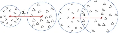
A novel nodes arrangement method based on fisher separability measure in feature space and margin of SVM is proposed to improve the above-mentioned drawbacks of DAGSVM. In order to reduce the risk of misclassification, the class which is easiest to distinguish should be separated preferentially and the secondary easy-to-distinguish class should be separated closely followed, the classes which are difficult to distinguish should be separated at last. This operation makes sure that the classification error appears at the bottom layer as much as possible, and then leads to the reduction of decision risk and accumulative error. Node arrangement method based on inter-class Euclidean distance is adopted first. It is obviously that the larger of the Euclidean distance between two classes of samples, the higher of the classifier position. However, when there are cross-distribution phenomena, Euclidean distance cannot evaluate separability of the classes effectively. This situation is shown in Figure 3, Euclidean distances are the same in the two diagrams, but obviously the classes in the left diagram are easier to separate.

ij

d

ij

d

Figure 3: Comparison Of Between-Class Separability With The Same Euclidean Distance

[image:6.612.316.514.584.640.2]

972

2 2

i j

ij

i j

c c d

δ δ

− =

+ (28)

where ci−cj is the distance between the ith class

and the jth class, and ci is the class-center of the ith

class, cj is the class-center of the jth class.

SVM deals with data in high dimensional feature space actually. The form of distribution of the data will be changed when the data are mapped to high dimensional feature space F by a nonlinear map

:x ( )x

φ φ ∈F from the original input space X , where X is a subset of n

R . Therefore, fisher separability measure in high dimensional feature space must be given firstly.

Fisher separability measure in high dimensional feature space is defined as

2 2

i j

ij

i j

C C

D = −

∆ + ∆ (29)

where Ciis the class-center of ith class in high

dimensional feature space, Cj is class-center of jth

class in high dimensional feature space, ∆2i and

2

j ∆

represent variance high dimensional in feature space.

1 1

( )

i

n

i is

s i

C x

n =φ

=

∑

(30)

1 1

( )

j

n

j jt

t j

C x

n = φ

=

∑

(31)

2 2

1 1

( ) 1

i

n

i is i

s i

x C

n = φ

∆ = −

−

∑

(32)

2 2

1 1

( ) 1

j

n

j jt j

t j

x C

n = φ

∆ = −

−

∑

(33)

Because the explicit expression of φis unknown, the formulas (30)-(33) cannot be solved directly. But, through the kernel function we can get Dij

directly without calculation of formulas (30)-(33). Obviously, Fisher distance Dij in feature space

can be obtained by a known kernel function ( , )x x

κ ′ _{, the separability of ith class and jth class}

can be judged. It can be seen from VC dimension and statistical learning theory that the larger the margin w is, the better the generalization performance of SVM, meaning better separability of two classes. Phetkaew realized this point first, and used it on selection of classification node. Therefore, in order to further reduce the classification risk, margin of different classes

2 w also should be considered.

For a k-class problem, take any combination of two in training phase like OAOSVM does, Ck2

bin-class bin-classifiers are constructed and each of them has a corresponding w . According to the formulas about separability measure in feature space, Ck2 Fisher separability measure can be

obtained. Consider margin 2 w _{and separability}

measure D, node arrangement principle of DAGSVM is given by formula (34).

2

2

2

1

1 (1 )

k

k

C i

i i

i i

C i

i w

D M

w

D

β = β

=

=

∑

+ −

∑

(34)

where i=1, 2,,Ck2. β∈[0.5,1].

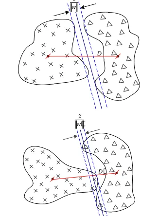
In order to reflect the importance of w , Figure 4 illustrates the reason for the setting range of

βschematically. The separability measures are the same (D=D′), however 2/|| ||w >2/|| ||w′ , thus the impact of margin is usually considered to be more important.

D

2 w

2 w

[image:7.612.336.481.405.627.2]

D

Figure 4: Comparison Of Margin With The Same Separability Measure

Firstly, M_i is arranged in descending order, then the node arrangement of DAGSVM can generally be determined by the sequence of Mi , from

ISSN: 1992-8645 www.jatit.org E-ISSN: 1817-3195

973 (IDAGSVM).

4. TWO-LEVEL STRUCTURE FOR FAULT

DIAGNOSIS AND EXPERIMENTAL RESULTS

4.1Two-level structure for fault diagnosis

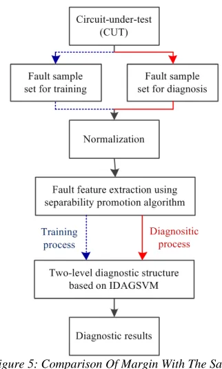
The flowchart of analog circuits fault diagnosis based on the proposed method is given in Figure 5, which includes two procedures, namely, the training procedure and the diagnosis procedure. First, the Monte Carlo simulation is performed for the fault-free circuit and faulty circuit respectively and the output responses have been randomly divided into two parts including training samples and testing samples. Then, we extract the nonlinear fault features of the circuit under test (CUT) using separability promotion algorithm from the training set and construct the diagnostic model which is based on IDAGSVM.

[image:8.612.338.485.257.525.2]

When performing fault diagnosis, we extract the corresponding major fault features from testing set and import the features to the diagnostic model that has been constructed. Then the IDAGSVM can assort all the fault classes of the CUT.

Figure 5: Comparison Of Margin With The Same Separability Measure

There are risks of false alarm and missing alarm in fault diagnosis system. We can tolerate the presence of the former to a certain extent, but usually we cannot accept the latter which could lead to tremendous loss. In order to reduce the risk

[image:8.612.112.273.392.659.2]

of false alarm and missing alarm, two-level diagnostic structure for analog circuit is proposed. In the first level, the training data is divided into two parts, including fault-free data (denoted as positive class points) and fault data (denoted as negative class points), then the labeled data is used to train the SVM. It is worth noting that such an approach will result in the unbalanced distribution of the training data in the first level. As shown in Figure 6, when the SVM is applied to dealing with class-unbalanced data, the generalized optimal separating hyperplane will be biased towards the majority class, thus causing poor diagnostic accuracy over the minority class.

Figure 6: Unbalanced Classification Problem Based On SVM

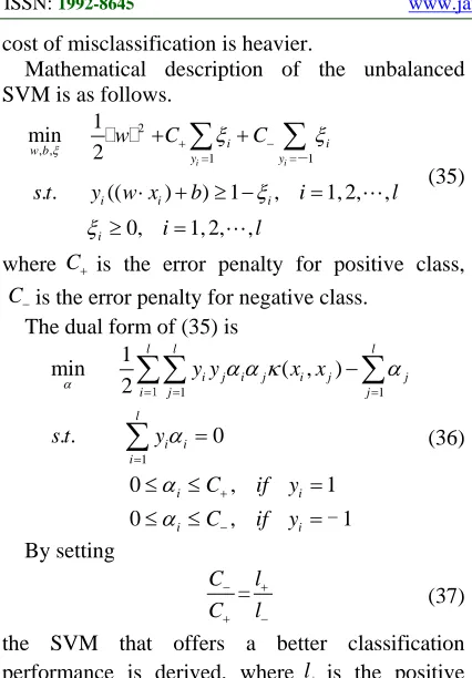
974 cost of misclassification is heavier.

Mathematical description of the unbalanced SVM is as follows.

2

, ,

=1 = 1

1 min

2

. . (( ) ) 1 , 1, 2, ,

0, 1, 2, ,

ξ ξ ξ

ξ ξ + − + + ⋅ + ≥ − = ≥ =

∑

∑

    － i i i i w b y y

i i i

i

w C C

s t y w x b i l

i l

(35)

where C+ is the error penalty for positive class,

C₋is the error penalty for negative class. The dual form of (35) is

1 1

1 1

min ( , )

2

. . 0

0 , 1

0 , 1

l l l

i j i j i j j

i j j

l

i i i

i i

i i

y y x x

s t y

C if y

C if y

α α α κ α

α α α = = = = + − − = ≤ ≤ = ≤ ≤ =

∑∑

∑

∑

１ (36) By setting = C l C l − + + − (37)

the SVM that offers a better classification performance is derived, where l₊ is the positive class size, l−is the negative class size. After the

first level of the diagnostic structure is achieved, the second level can be determined by the sequence of Mi.

4.2Diagnostic Flowchart

To verify the efficiency of the method proposed in this paper, ITC benchmark analog circuit leap-frog filter [15] is taken as the CUT. The circuit schematic and nominal values of the components are shown in Figure 7, the resistors and capacitors are assumed to have tolerances of 10% and 5%, respectively. Pspice tool is used to simulate this circuit.

+ −

+ −

4(10 ) R k

7(10 ) R k

3(0.02 ) C µF

+ −

8(10 ) R k

5(10 ) R k 2(10 )

R k

1(0.01 ) C µF 1(10 )

R k

in

V

+ −

2(0.02 ) C µF

+ −

9(10 ) R k

11(10 )

R k +

−

10(10 ) R k

4(0.02 ) C µF 12(10 )

R k 3(10 ) R k out V 5 V 1 V 2

V V3

6(10 ) R k

4

V

6

V V7

8

V

10

V V11 9

V

12

[image:9.612.89.302.80.386.2]

V

Figure 7: Leap-Frog Filter

[image:9.612.312.521.226.406.2]

All the parameters in the circuit are varied within the tolerance range and Monte Carlo simulation is performed for both fault-free and faulty circuit. After 200 Monte Carlo simulations, the output responses have been randomly divided into two parts including 120 training samples and 80 testing samples. The fault classes and the faulty component values are listed in Table 1, where ↑ and ↓ imply significantly higher or lower than nominal value.

Table 1: Fault Classes Of Leap-Frog Filter

Fault code Fault class Nominal value Faulty value

F0 Fault-free — —

F1 C1↓ 0.01μF 0.005μF

F2 C1↑ 0.01μF 0.015μF

F3 C2↓ 0.02μF 0.01μF

F4 C2↑ 0.02μF 0.03μF

F5 C3↓ 0.02μF 0.01μF

F6 C3↑ 0.02μF 0.03μF

F7 C4↓ 0.02μF 0.01μF

F8 C4↑ 0.02μF 0.03μF

F9 R1↓ 10kΩ 5kΩ

F10 R2↓ 10kΩ 6kΩ

F11 R3↓ 10kΩ 7kΩ

F12 R4↑ 10kΩ 13kΩ

F13 R5↑ 10kΩ 14kΩ

F14 R10↓ 10kΩ 7kΩ

F15 R11↓ 10kΩ 8kΩ

F16 R12↑ 10kΩ 15kΩ

In our experiment, Gaussian kernel function

2 2

( , )x y exp( ||x y|| /2 )

κ = − − σ is adopted and the

selection range of regularization parameter c is

4 2 12

[2 , 2 ,− − , 2 ] , the selection range of σ2 _in Gaussian kernel function is 10 9 8

[2− , 2 ,− , 2 ]. The sampled data are preprocessed by separability promotion algorithm for nonlinear feature extraction. Then the nonlinear features extracted from the test samples together with their labels are fed into the two-level diagnostic structure whose outputs estimate the probabilities that input features belong to different fault classes. The contribution rates of the first 10 KPCs for KPCA are listed in Table 2.

Table 2 : The Contribution Rates Of Kpcs

Kernel principal Eigenvalue Contribution rate

KPC1 9.97 35.02%

KPC2 7.55 26.52%

KPC3 4.75 16.68%

KPC4 2.86 10.05%

KPC5 1.68 5.90%

KPC6 0.89 3.13%

KPC7 0.43 1.51%

KPC8 0.21 0.74%

KPC9 0.09 0.32%

[image:9.612.310.522.605.719.2]

ISSN: 1992-8645 www.jatit.org E-ISSN: 1817-3195

[image:10.612.106.528.69.519.2]

975 It can be seen from Figure 8 that the cumulative percent variance (CPV) of the first 5 KPCs is 94.17% in excess of 85%. At this point, it can be accounted that most of the nonlinear feature information has been extracted. The scatter diagrams of all kinds of fault features extracted by separability promotion algorithm are shown in Figure 9-12.

[image:10.612.124.267.202.322.2]

Figure 8: Cumulative Percent Variance

[image:10.612.123.273.356.482.2]

Figure 9: Two Dimensional Reconstructed Data Of Fault Classes With Odd Coding

Figure 10: Three Dimensional Reconstructed Data Of Fault Classes With Odd Coding

Figure 11: Two Dimensional Reconstructed Data Of Fault Classes With Even Coding

[image:10.612.311.524.417.597.2]

Figure 12: Three Dimensional Reconstructed Data Of Fault Classes With Even Coding

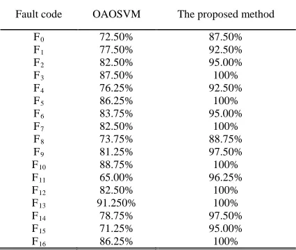
Table 3 : Diagnostic Accuracy Of The CUT

Fault code OAOSVM The proposed method

F0 72.50% 87.50%

F1 77.50% 92.50%

F2 82.50% 95.00%

F3 87.50% 100%

F4 76.25% 92.50%

F5 86.25% 100%

F6 83.75% 95.00%

F7 82.50% 100%

F8 73.75% 88.75%

F9 81.25% 97.50%

F10 88.75% 100%

F11 65.00% 96.25%

F12 82.50% 100%

F13 91.250% 100%

F14 78.75% 97.50%

F15 71.25% 95.00%

F16 86.25% 100%

[image:10.612.117.275.518.643.2]

976

5. CONCLUSION

Fault diagnosis of analog circuit is of essential importance for guaranteeing the reliability and maintainability of electronic systems. Two-level diagnostic structure for faulty analog circuit is proposed in this paper. In order to overcome the shortcomings of DAGSVM, the improved strategies based on fisher separability measure in feature space and margin of SVM is proposed. Then the separability promotion algorithm based on KPCA plus LDA is proposed and used to extract the nonlinear fault features. The experimental results show that it has a significant impact on analog circuits fault diagnosis, due to the excellent ability of nonlinear features extraction. Meanwhile, it can enhance class separability and reduce the within-class scatter in high dimensional space. Consequently, the purpose of improving the diagnostic accuracy is achieved.

ACKNOWLEDGEMENTS

This work was supported by NSFC (61074127).

REFERENCES:

[1] H. Luo, Y. Wang, Jiang Cui. “A vague decision method for analog circuit fault diagnosis based on description sphere”, Chinese Journal of

Aeronautics, Vol. 24, No. 6, 2011, pp. 768-776.

[2] F. Li, Y. P. Woo. “Fault detection for linear analog IC—The method of short-circuit admittance parameters”, IEEE Transactions on Circuits and Systems I: Fundamental Theory

and Applications, Vol. 41, No. 9, 2002, pp.

105-108.

[3] W. G. Fenton, T. M. McGinnity, L. P. Maguire. “Fault Diagnosis of Electronic Systems Using Intelligent Techniques: A Review”, IEEE Transactions on Systems, Man, and Cybernetics

—Part C: Applications and Reviews, Vol. 31,

No. 3, 2001, pp. 269-281.

[4] Y. Xiao, Y. He. “A novel approach for analog fault diagnosis based on neural networks and improved kernel PCA”, Neurocomputing, Vol. 74, No. 7, 2011, pp. 1102-1115.

[5] R. Spina, S. Upadhyaya. “Linear circuit fault diagnosis using neuromorphic analyzers”, IEEE Transactions on Circuits and Systems II:

Analog and Digital Signal Processing, Vol. 4,

No. 3, 1997, pp. 188-196.

[6] M. Aminian, F. Aminian. “Neural-network based analog circuit fault diagnosis using wavelet transform as preprocessor”, IEEE Transactions on Instrumentation and

Measurement, Vol. 51, No. 3, 2002, pp.

544-550.

[7] M. Aminian, F. Aminian. “Neural network based analog circuit fault diagnosis using wavelet transform as preprocessor”, IEEE Transactions on Circuits and Systems II:

Analog and Digital Signal Processing, Vol. 47,

No. 2, 2000, pp. 151-156.

[8] Y. Xiao, L. Feng. “A novel neural-network approach of analog fault diagnosis based on kernel discriminant analysis and particle swarm optimization”, Applied Soft Computing, Vol. 12, No. 2, 2012, pp. 904-920.

[9] Y. Wang, J Cui. “A novel approach of analog circuit fault diagnosis using support vector machines classifier”, Measurement, Vol. 44, No. 1, 2011, pp. 281-289.

[10] H. Luo, Y. Wang, J. Cui. “A SVDD approach of fuzzy classification for analog circuit fault diagnosis with FWT as preprocessor”, Expert

Systems with Applications, Vol. 38, No. 8,

2011, pp. 10554-10561.

[11] Z. Yang, Y. Peng, X. Peng. “Research on classification technique for imbalanced data set based on support vector machines”, Chinese

Journal of Scientific Instrument, Vol. 30, No. 5,

2008, pp. 1094-1099.

[12] B. Schölkopf, A Smola. “Nonlinear component analysis as a kernel eigenvalue problem”,

Neural Computation, Vol. 10, No. 6, 1998, pp.

1299-1319.

[13] H. Gao, J. W. Davis. “Why direct LDA is not equivalent to LDA”, Pattern Recognition, Vol. 39, No. 5, 2006, pp. 1002-1006.

[14] C. Hsu, C. Lin. “A comparison of methods for multiclass support vector machines”, IEEE

Transactions on Neural Networks, Vol. 13, No.

2, 2002, pp. 415-425.

[15] J. Roh, J. A. Abraham. “Subband filtering for time and frequency analysis of mixed-signal circuit testing”, IEEE Transactions on

Instrumentation and Measurement, Vol. 53,