Copyright by Duehee Lee
The Dissertation Committee for Duehee Lee
certifies that this is the approved version of the following dissertation:
Wind Power Forecasting and Its Applications to the
Power System
Committee:
Ross Baldick, Supervisor Surya Santoso
Aristotle Arapostathis Michael Webber David Morton
Wind Power Forecasting and Its Applications to the
Power System
by
Duehee Lee, B.S.; M.S.E.
DISSERTATION
Presented to the Faculty of the Graduate School of The University of Texas at Austin
in Partial Fulfillment of the Requirements
for the Degree of
DOCTOR OF PHILOSOPHY
THE UNIVERSITY OF TEXAS AT AUSTIN May 2015
Dedicated to my wife Jain Hong, my son James Lee, and my daughter Jacqueline Lee.
Acknowledgments
First, I would like to express my deepest gratitude to my supervisor, Dr. Ross Baldick for his support, encouragement, and suggestions. Under his guidance, I have gained the courage to tackle any research topic. When I had no place to go, he led me toward studying the power system. He has taught me the power system protocol, how to behave in the academic field, and how to endure hard times.
I would like to thank my wife for enduring poverty, parenting, and uncertainty with me. I promise that I will be her strong supporter when she passes the same thorny path. My gratitude also goes to my other family members: my father, sister, grandfather, mother-in-law, and father-in-law.
I am also indebted to my dissertation committee members, Dr. Aristo-tle Arapostathis, Dr. David Morton, Dr. Michael Webber, and Dr. Surya toso. In particular, I would also like to thank my former supervisor Surya San-toso for his invaluable comments, support, and help in studying wind power. Furthermore, without the support of Carey King, Mack Grady, and Melanie Gulick, this dissertation would not have been written. I should not forget my English teacher, Meg Downing. She has been a friend with whom to talk about life in Austin, an editor, and a colleague with whom to discuss various research topics. I hope that she and her family are healthy, happy, and prosperous.
I wish to thank to all my Korean friends in our energy system, Joon-hyun Kim, Youngsung Kyun, Myungchin Kim, Cheolhee Cho, Hunyoung Shin, Sungwoo Bae, Seunghyun Chun, Jin hur, Wonjin Cho, Seounghoon Jung, Byungchul Lee, Myungkwan Kim, Joohyun Jin, Han Kang, Kyungwoo Min, Wanki Cho, and Kwangmin Choi. I also owe my deepest gratitude to my older brothers and sisters at UT, Jinho Lee, Youngsuck Yoo, Peter Son, Mijung Park, Woori Kim, Mooryong Choi, Il Memming Park, Manho Jung, Hur Kyun, Yea-joon Kim, Youngchoon Kim, and Larkkwon Choi. I also wish to thank all my alumni friends, Byungchul Lee, Insoo Hwang, Jaewon Kim, Solkun Jee, Insun Cho, Jaehyun Bae, Jaewook Lee, Sungmin Oak, and Hoo Kim.
Friends in my research group are my comrades. We have dreamed the same dream, studied the same topics, and corresponded a lot. I will never for-get Bowen Wa, Hector Chavez, Yezhou Wang, Yen-yu Lee, David Tuttle, Thuy Huynh, Deepjyoti Deka, Sambuddha Chakrabarti, Tong Jang, Juan Andrade, Mohammad Majidi, Mansoureh Peydayesh, and Michael Legatt.
Importantly, I would like to express my gratitude to other friends, Kijung Yoon, Juhun Lee, Gerad Garrison, Mohit Singh, Alicia Allen, Min Lwin, Swagata Das, Anamika Dubey, Pisitpol Chirapongsananurak, David Orn, Twoone Ngo, Quan, Suma Jothibasu, Jules Campbell, Marcel Nas-sar, Kyungjin Kim, Neeraj Karnik, Yaidy Viswanadan, Hose Caso, Fernando Ochoa, Kai Roach, and Michael Pinnel. Finally, I want to deliver my grati-tude to all my friends who know me but who are not mentioned on this page. Although they are not mentioned here, we have been and will be together.
Wind Power Forecasting and Its Applications to the
Power System
Publication No.
Duehee Lee, Ph.D.
The University of Texas at Austin, 2015
Supervisor: Ross Baldick
The goal of research in this dissertation is to bring more wind resources into the power grid by mitigating the uncertainty of the current wind power, by developing a new algorithm to respond to the fluctuation of the future wind power, and by building additional transmission lines to bring more wind re-sources from a remote area to the load center. First, in order to overcome the wind power uncertainty, the probabilistic and ensemble wind power forecasting is proposed to increase the forecasting accuracy and to deliver the probability density function of the uncertainty. Accurate wind power forecasting reduces the amounts and cost of ancillary services (AS). As the mismatch between the bid and actual amount of delivered energy decreases, the imbalance between supply and demand also decreases. If the forecasting ahead is increased up to 24 hours, accurate wind power forecasting can also help wind farm owners bid the exact amount of wind power in the day ahead (DA) market.
Further-more, wind power owners can use the parametric probabilistic density of error distributions for hedging the price risk and building a better offer curve.
Second, a novel algorithm to generate many wind power scenarios as a function of installed capacity of wind power is proposed based on an analysis of the power spectral density of wind power. Scenarios can be used to simulate the power system to estimate the required amount of AS to respond to the fluctuation of future wind power as the installed capacity of wind power in-creases. Scenarios have statistical characteristics of the future wind power that are regressed as a function of the installed capacity of wind power from the statistical characteristics of the current wind power. This algorithm can gen-erate many possible scenarios to simulate the power system in many different situations.
Third, optimal transmission expansion by simulating the power sys-tem with the multiple load and wind power scenarios in different locations is planned to prepare the preliminary result to bring more wind resources in remote areas to the load center in Texas. In this process, the geographical smoothing effects of wind power and the stochastic correlation structure be-tween the load and wind power are considered. Furthermore, the generalized dynamic factor model (GDFM) is used to synthesize load and wind power scenarios to keep their correlation structure. The premise of the GDFM is that a few factors can drive the correlated movements of load and wind power simultaneously, so the scenario generation process is parsimonious.
Table of Contents
Acknowledgments v
Abstract vii
List of Tables xiii
List of Figures xiv
Chapter 1. Introduction 1
1.1 Wind Power in the Electricity Market . . . 2
1.1.1 Benefits of Wind Power . . . 2
1.1.2 Economic Incentives for Wind Power . . . 3
1.1.3 Wind Power As an Electricity Market Participant . . . . 4
1.1.4 Effect on the Power System and Electricity Market . . . 6
1.2 Solutions to Increase the Wind Power Capacity . . . 10
1.2.1 Advanced Ancillary Services Procurement Process . . . 10
1.2.2 Storage System . . . 11
1.2.3 Electric Vehicles . . . 12
1.2.4 Wind Power Forecasting . . . 13
1.2.5 Transmission Expansion . . . 14
1.3 Motivation and Goals . . . 15
1.4 Organization . . . 21
Chapter 2. Short-Term Wind Power Forecasting 22 2.1 Introduction . . . 24
2.1.1 Literature Review . . . 25
2.1.2 Global Energy Forecasting Competition . . . 27
2.2 Program Architecture . . . 28
2.2.2 Internal Forecasting . . . 29 2.2.3 First Stage . . . 31 2.2.4 Second Stage . . . 34 2.2.5 Third Stage . . . 34 2.3 Feature Engineering . . . 35 2.3.1 Data Smoothing . . . 36 2.3.2 Data Transformation . . . 37 2.3.3 Data Expansion . . . 37 2.3.4 Outlier Detection . . . 38
2.3.5 Input Data Classification . . . 38
2.3.6 Pre-processing and Post-processing . . . 39
2.3.7 Simulation Settings for Individual Forecasting Machines 40 2.4 Forecasting Machines . . . 40
2.4.1 Ridge Regressions . . . 41
2.4.2 Neural Network . . . 42
2.4.3 Support Vector Machines . . . 45
2.4.4 Gaussian Process . . . 46
2.4.5 Bootstrap Aggregation (BAG) . . . 48
2.4.6 Random Forest . . . 49
2.4.7 Gradient Boosting Machines . . . 51
2.5 Ensemble Forecasting . . . 54
2.5.1 Analysis of Individual Forecasting Machines . . . 54
2.5.2 Ensemble Algorithms . . . 56
2.6 Quantile Estimation . . . 57
2.6.1 Pinball Loss Function . . . 58
2.6.2 Probabilistic Forecasting in the Ensemble Forecasting . 59 2.6.3 Parametric Approach . . . 59
2.6.4 Distributions . . . 61
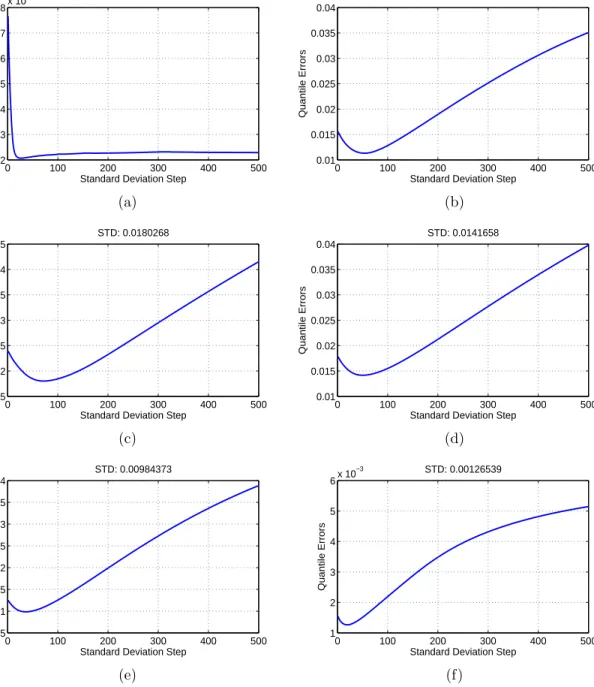
2.6.5 Estimation of the Standard Deviations: Discrete Cluster Case . . . 64
2.6.6 Point Forecast Clustering . . . 65
2.6.8 Estimation of the Standard Deviations: Continuous Case 67
2.6.9 Simulation Results . . . 69
2.7 Conclusions . . . 71
Chapter 3. Total Future Wind Power Scenario Generation 74 3.1 Introduction . . . 75
3.1.1 Literature Review . . . 76
3.1.2 Preprocessing . . . 79
3.2 Power Spectral Density Estimation . . . 80
3.2.1 Periodogram . . . 81
3.2.2 Multitaper Algorithm . . . 83
3.3 Piecewise Modeling of the PSD . . . 86
3.3.1 Hinges Model . . . 86
3.3.2 Original Hinges Model . . . 87
3.3.3 Modified Hinges Model . . . 91
3.4 Training Data Generation . . . 92
3.4.1 Factor Analysis . . . 94
3.4.2 Cluster Analysis . . . 97
3.5 Wind Power Ramp Modeling . . . 97
3.6 Analysis of Slopes . . . 99
3.6.1 Wind Power Fluctuation . . . 99
3.6.2 Slope Change Analysis . . . 103
3.6.3 Regression . . . 105
3.7 Scenario Synthesis . . . 109
3.7.1 PSD Forecasting . . . 111
3.7.2 Phase Angle Generation . . . 112
3.7.3 Genetic Algorithm . . . 113
3.7.4 Phase Angle Analysis . . . 115
3.8 Validation . . . 115
3.9 Ancillary Service Estimation . . . 123
3.10 Conclusion . . . 125
Chapter 4. Scenario Generation through GDFM and
Transmis-sion ExpanTransmis-sion Planning 127
4.1 Literature Review . . . 128
4.2 Additional Motivations and Goals . . . 132
4.3 Preprocessing and the GDFM . . . 133
4.3.1 Preprocessing Wind Power & Load Data . . . 134
4.3.2 Introduction to the GDFM . . . 134
4.3.3 Decomposition . . . 137
4.3.4 Estimation . . . 139
4.4 Load and wind power Scenario Generation . . . 141
4.4.1 Number of Dynamic Factors . . . 142
4.4.2 Scenario Generation . . . 142
4.4.3 Statistics & PSD Analysis . . . 145
4.4.4 Correlation Coefficient . . . 147
4.5 Generation & Transmission Upgrading Costs . . . 152
4.5.1 Simulation Settings . . . 153
4.5.2 Simulation Results . . . 154
4.6 Conclusion . . . 156
Chapter 5. Conclusion 157 5.1 Short-Term Wind Power Forecasting . . . 157
5.1.1 Key Results . . . 158
5.1.2 Future Work . . . 159
5.2 Long-Term Wind Power Scenario Generation . . . 159
5.2.1 Key Results . . . 160
5.2.2 Future Work . . . 161
5.3 Load and Wind Power Scenario Generation and Transmission Expansion Planning . . . 162
5.3.1 Key Results . . . 163
5.3.2 Future Work . . . 164
Bibliography 165
List of Tables
1.1 Wind Power in Electricity Markets . . . 7
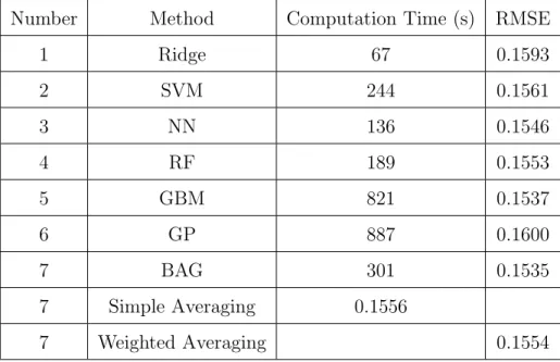
2.1 Performance of forecasting machines. . . 56
2.2 Performance of the quantile estimation methods . . . 70
3.1 Frequency-axis hinge locations . . . 92
3.2 Statistical characteristics of actual and synthesized wind power 124 4.1 Evaluation of Statistical Characteristics . . . 150
List of Figures
2.1 Forecasting unit . . . 24
2.2 Three-stage program architecture . . . 30
2.3 Program architecture of five for-loops . . . 32
2.4 Forecasting process of individual step . . . 33
2.5 Correlation coefficients of transformed features . . . 36
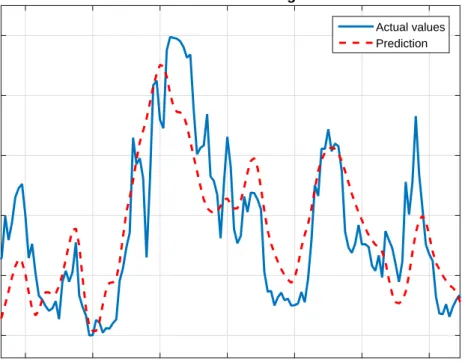
2.6 Example of wind power forecasting . . . 43
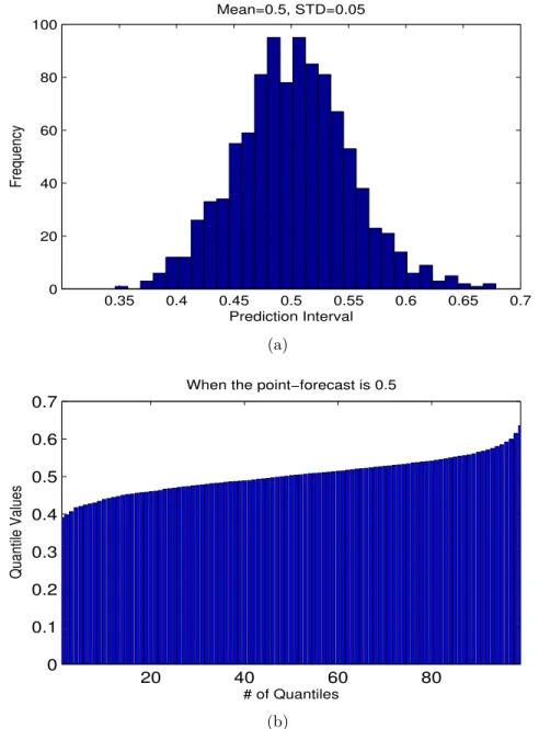
2.7 The Gaussian distribution and its quantile function . . . 60
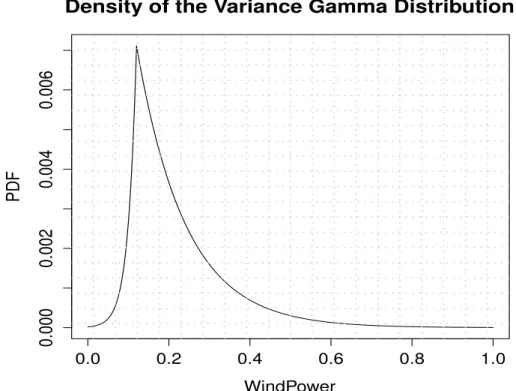
2.8 The variance gamma distribution . . . 63
2.9 Quantile errors with respect to the STDs for different groups . 66 2.10 Data clustering . . . 68
2.11 A truncated VG distribution . . . 69
3.1 The PSD of wind power and its six slopes . . . 88
3.2 Wind power and its smoothed wind power . . . 98
3.3 The variability of un-normalized wind power . . . 100
3.4 Initial and final values of PSD . . . 101
3.5 Slope changes according to the number of wind farms . . . 103
3.6 Histogram of the power difference . . . 104
3.7 Slopes of first and second segments . . . 106
3.8 Slopes of third and fourth segments . . . 107
3.9 Slopes of fifth and sixth segments . . . 110
3.10 The means of the STDs of phase angles per frequency. . . 116
3.11 The actual wind power scenario sampled in April 2010. . . 117
3.12 The wind power scenario in 2010 based on the wind power in 2009 . . . 118
3.13 The wind power scenario in 2010 based on the wind power in 2010 . . . 119 3.14 The wind power scenario of 10,000 MW installed capacity in 2030120
3.15 Actual distributions of wind power ramp rate and phase angle 121 3.16 Distributions of ramp rates and phase angles of synthesized
wind power scenarios . . . 122
4.1 Coastal load data and common component . . . 143
4.2 Wind power data and common component . . . 144
4.3 Coastal load data and new scenario . . . 146
4.4 Wind power data and new scenario . . . 147
4.5 PSD of actual load data . . . 148
4.6 PSD of actual wind power data . . . 149
4.7 The correlation coefficients of actual waveforms . . . 151
Chapter 1
Introduction
Electric energy comes from many primary energy resources. One of those energy sources is wind energy although strictly speaking wind energy itself is primarily due to energy from the sun. In the Electric Reliability Council of Texas (ERCOT), of the 340,033,353 MWh annual total electrical energy produced in 2014, 36,142,384 MWh, or 10.6% of annual total electrical energy, came from wind energy [65]. Furthermore, the installed wind power capacity comprised 14% of the total installed capacity of generators, and the maximum generation of wind power was 10,957 MW on December 25, 2014, which comprised 34% of total demand. The total installed wind power capacity might increase in 2015 because about 3,000 MW of additional wind power is under an interconnection agreement [64].
In comparison, in 2008, wind energy comprised 2.9% of total annual energy, and the capacity provided by wind power comprised just 7.1% of total installed capacity [61]. It is clear that wind energy has increased tremendously between 2008 and 2014. Why have many companies invested in wind resources, what are the advantages and disadvantages of bringing more wind power into our power system, and how can we mitigate its disadvantages and emphasize
the advantages? The answers for the first two questions are briefly answered in this chapter. The rest of this dissertation aims to answer the last question.
1.1
Wind Power in the Electricity Market
The explosive increase of wind energy in the U.S. has been encouraged by the efforts of the federal and state governments to take advantage of the benefits of wind power. These efforts have been realized through various eco-nomic incentives in order to facilitate the appropriate market environment for wind farm owners and wind turbine generating companies.
1.1.1 Benefits of Wind Power
There are five main benefits of wind energy. 1) Wind energy is sustain-able as long as the wind blows. 2) Since wind energy is a domestic resource that does not need to be mined and transported, the U.S. can increase en-ergy independence and diversify its enen-ergy portfolio in order to respond to the changeable international energy market. 3) Wind turbines generate negligible amounts of atmospheric emissions that cause greenhouse effects. Reducing the greenhouse gas emissions can delay the greenhouse effect. 4) Since good wind sites are often in remote areas, the rural area can benefit from increased prop-erty taxes and direct lease payments. Moreover, land used for wind farms can still be used for agriculture. 5) Wind turbines do not require large amounts of water, in contrast to nuclear power and coal power [128]. In generating the same amount of energy, a nuclear power plant requires 500 times more water
than a wind turbine does.
In spite of these benefits, the leveled cost of wind energy in dollars per MWh is still higher than that of other energy resources. For example, the levelized cost of offshore and onshore wind power is $204/MWh and $80/MWh, respectively although recent costs have declined somewhat [3]. In contrast, the levelized cost of natural gas combined cycle generator is $64/MWh. Therefore, in order to realize the benefits of wind energy, it is necessary to facilitate the participation of wind energy in the electricity market through various economic incentives.
Before introducing the economic incentives for wind energy, it should be noted that the development of renewable energy has also been spurred by state governments by setting specific and mandatory target amounts of renewable energy, which is called the renewable portfolio standard (RPS) [94]. The RPS is defined as the target capacity of renewable energy by the target year, or the target percentage of the capacity of renewable energy with respect to the load capacity. For example, in Texas, the RPS target is 10,000 MW by 2025, and it has already been achieved. The economic incentives that will be explained below have played an important role in satisfying the RPS.
1.1.2 Economic Incentives for Wind Power
There are three economic incentives for wind power. 1) The marginal cost of wind power is almost zero, so wind power is typically dispatched in preference to all other resources in an electricity market. In fact, wind farm
owners sometimes bid at negative prices due to other incentives that will be explained below. 2) The federal government gives tax incentives to promote renewable energy businesses: wind farm owners are eligible for a production tax credit (PTC) of 2.3 cents perkW h generated for the first ten years. Be-cause of the PTC, nearly $15 billion was invested in wind power between 2007 and 2014 in the U.S [114]. It should be mentioned that the PTC expired on December 31, 2013, so new wind resources built after 2014 are not currently eligible, but debate about the extension is on-going. 3) Wind farm owners can earn a renewable energy certificate (REC) by selling one MWh. The REC can be sold in two types of REC markets, the voluntary and the compliance markets, and the price is always changing according to the year, the type of REC market, and the state in which the REC is sold. In the voluntary REC market, many companies buy voluntary RECs to show that they are environ-mentally friendly, and in the compliance REC market, the RECs are sold to load entities in each state to satisfy the RPS.
1.1.3 Wind Power As an Electricity Market Participant
As a result of the above-described incentives, wind power has expanded in the electricity market. However, it has been difficult to handle wind power in the same manner as conventional power because of wind power’s uncertainty and fluctuation. Since the wind power is generally determined by wind speed, which cannot be predicted with 100% accuracy, the wind power prediction always has a natural uncertainty. In addition, since wind farm owners cannot
control the intermittent nature of wind, the wind power output always fluctu-ates with various ramp rfluctu-ates, although modern wind turbines can control the ramp rates of wind power penetration to a certain extent.
Because of these two distinguishing characteristics of wind power, as compared with other generators, relaxed or different market rules have been applied to wind power in various electricity markets in the U.S. For example, in the New York ISO (NYISO), there is a penalty for non-compliance to the dis-patch point outside a 3% margin of error, and the cost of the penalty is the mul-tiplication of the deviation amount and the regulation clearing price. However, up to 3,300 MW of installed wind capacity is exempt from under-generation penalties. In the Midwest ISO (MISO), wind power, which is considered as the dispatchable intermittent resource (DIR), follows different market rules compared to conventional generators. For example, DIRs are exempted for deviations less than 30 MWh. In ERCOT, wind producers are only penalized if wind power deviates above the expected point, but not for the deviation below. If wind power deviates more than 10% above the expected point, it will be charged based on the real-time (RT) price and power balance penalty curve, and wind power cannot ramp more than 10% of its capacity within a minute. On the contrary, conventional generators are fined when their gen-eration outputs deviate more than 5% above or below the expected point. Moreover, wind power is not allowed to participate in the ancillary service market. The different wind power market rules in different ISOs are summa-rized in Table 1.1.
Generally, participation in the RT market and acceptance of the dis-patch signal is mandatory in most ISOs, but participation in the day-ahead (DA) market is voluntary. Furthermore, most ISOs allow a negative price. If wind power is used to provide the capacity resource, particularly in Pennsyl-vania New Jersey Maryland Interconnection (PJM) market, then wind farm owners should offer the capacity resource in the DA market. In PJM, wind receives capacity credit based on a average of performance over the previous three summers. If the operation duration is less than three years, wind power receives 13 percent of nameplate capability [187]. For the unit commitment, which decides when generators should be turned on and off, wind power is just considered as a negative load, and the wind power variability is represented as the net load (load – wind) variability. Sometimes, as in MISO, PJM, and ERCOT, wind power is curtailed because of transmission constraints or the minimum generation events. In ERCOT in particular, wind power is often curtailed because of insufficient capacity of the transmission lines that deliver much of the wind energy from West Texas to the load centers. In addition, the centralized wind power forecasting has been used to dispatch wind power and determine the amounts of regulation services to be procured in various electricity markets.
1.1.4 Effect on the Power System and Electricity Market
The introduction of wind power might affect the power system in terms of the wholesale electricity price, system inertia, and amounts of AS. However,
Table 1.1: Wind Power in Electricity Markets
Electricity Market PJM NYISO ERCOT
Dispatch Must participate in the RT market.
Must participate in the RT market.
Must participate in the RT market. Day Ahead Market Only as a
capac-ity resource, wind power must bid in the DA market.
Voluntary Voluntary
Negative Price Allowed Allowed Allowed
Imbalance Relaxation Costs are charged for power imbal-ance.
Wind power is ex-empt from under-generation penalty up to 3,300 MW of installed capacity of wind power During testing periods, if wind resource gener-ates more than 10% above, it will be charged on real-time prices. AS Market Can participate
only in the regula-tion market.
Can participate only in the regula-tion market. Can participate in the frequency response without payment. Can provide regulation service.
Forecasting System Since 2009. Long term: hourly from 48 hours ahead to 168 hours ahead. Medium term: hourly from 6 hours ahead to 48 hours ahead. Short Term: at every 10 min with forecast interval of 5 min for next 6 hours.
It has been used since 2008. The DA forecasting is pro-vided twice in a day (4am, 4pm), and the RT forecasting is provided at every 15 min.
It has been used since 2008. Hourly wind power fore-casting also pro-vides 50% and 80% probabilities of over-forecast for 48 hours.
Ramp Forecasting Updated every 10 minutes at 5-min intervals for next 6 hours.
No ramp forecast Probabilistic ramp forecasting is pro-vided at every 15 min for the upcom-ing 6 hours.
determining the direct impact of wind power on the wholesale price might be difficult because the wholesale prices are also affected by weather, natural gas prices, transmission constraints, load, and other factors. The wholesale price in 2012 was lower than the price in 2008. Low natural gas prices and electricity demand are considered to be two primary contributors to this decrease. How-ever, it is true that wind power can potentially reduce wholesale electricity prices since its marginal cost is close to zero, and wind power is sometimes bid with a negative price. Therefore, the strong impact of wind power on the wholesale price has not been clearly shown, but it will contribute to a decrease in the wholesale price as the wind power penetration level increases. Additional transmission lines might decrease the wholesale price further by delivering more wind power to the grid.
Another effect that wind energy might have on the power system is re-garding the system inertia. The system inertia decreases as more wind farms are integrated into the power system. The inertia is an index to describe the sum of all kinetic energy in the on-line synchronous generators that are run-ning with the same 60 Hz frequency. By following Newton’s first law, the inertia delays the frequency deviation from 60 Hz when there is a power im-balance between the supply and demand [139]. On the contrary, most wind turbines, which are inverter-based generators or asynchronous induction gen-erators, are not synchronized with other generators at 60 Hz, so they cannot directly provide the inertia to the power system. With reduced inertia, the system frequency drops faster after a generator contingency than the system
frequency with normal system inertia, so more responsive services are required to delay the frequency drop in the system with less system inertia. Although wind turbines can also provide synthetic inertia, since they require a control action triggered by the system frequency drop, a market-based procurement process would likely need to be established in order for wind farm owners to provide this service.
In addition to affecting the system inertia, increased wind capacity might also increase the amount of regulation services, which are deployed to compensate for the power imbalance within each five minute dispatch inter-val, because the wind power fluctuation within the five minutes can increase the net load fluctuation. However, the effect of increased wind capacity on the amounts of ancillary services (AS) has not been shown clearly yet because ISOs have changed their regulation procurement methodologies as the penetration level of wind power has increased. PJM has reported that there have been no serious impacts of wind power on the procured amount of regulation services. Although ERCOT’s current regulation procurement methodology is also ade-quate to procure sufficient regulation services [195], ERCOT has increased the procured amounts of regulation services with respect to the installed capacity of wind power by following the guidelines in [195].
Furthermore, wind power forecasting has been used for calculating the amounts of non-spinning reserve services more accurately. The load and wind power forecast uncertainties are used to calculate the net load uncertainty and thus the amount of hourly non-spinning reserve services. Therefore,
in-creased wind capacity might increase the amount of regulation services, and the improved performance of wind power forecasting is required to estimate the amounts of non-spinning reserve services more accurately.
1.2
Solutions to Increase the Wind Power Capacity
Three obstacles to increase the penetration level of wind power are wind power fluctuation preventing participation in the DA market where prices are less volatile and higher than the RT market, the increasing cost of AS, and limited transmission resources. There are three key solutions to these ob-stacles: promoting participation of wind power providers in the AS and DA markets by improving the wind power forecasting and developing the stor-age system, developing smart AS procurement methodologies, and building additional transmission lines.
1.2.1 Advanced Ancillary Services Procurement Process
As the wind capacity increases, the optimal amounts of AS, respon-sive services, regulation services, and non-spinning services can be procured based on the installed wind capacity, the inertia, governor response ramp rate, droop-characteristic, and net load variability [42]. In order to compensate for the decreasing inertial response capability, a new process to procure the responsive service can be determined by considering governor response ramp rates and system inertia so that the responsive service stabilizes the frequency when a generator trips [43]. The amounts and ramping capability of
regu-lation services can also be set with respect to the net load variability while satisfying the Control Performance Standard (CPS) [44]. As the wind pen-etration level increases, the absolute magnitude of net load variability also increases, so the required regulation service is also expected to increase. Al-though wind turbines can only provide down regulation, curtailment of wind power to provide the down regulation might erode the low-cost advantage of wind power. The non-spinning service, which compensates for net load vari-ability and recovers the 60Hz frequency after the resources are deployed, can be upgraded to procure resources by considering the ramp rates of resources. For example, ERCOT plans to substitute the current non-spinning service for the supplemental reserve (SR) service. It should be noted that ERCOT’s new AS system includes six different services: synchronous inertial response (SIR), fast frequency response (FFR), primary frequency response, up and down reg-ulating reserve, contingency reserve, and SR services [63].
1.2.2 Storage System
Participation in the DA and AS markets can be expanded through the use of the storage systems, which will mitigate the effect of wind power fluctu-ation and reduce the exposure of wind farm owners to the volatile price in the RT market. The storage system can also be used to relieve the transmission congestion of wind power, mitigate wind power fluctuation, and provide AS. A large capacity storage system, such as the compressed air energy storage (CAES), can relieve the transmission congestion due to wind power if it is
installed around the transmission lines and wind farms. Furthermore, by lim-iting the ramp rate of wind power, the storage system can mitigate the wind power fluctuation. For example, Xtreme Power installed a storage system of 10 MW power rating and 20MWh storage size on a 21 MW wind farm in Maui, Hawaii to limit the ramp rates of wind power. The ramp rate limit was ±1 MW / min. Xtreme Power’s storage system can also provide the regula-tion service because it can respond to the regularegula-tion signal very quickly [172]. ERCOT has a plan to introduce the storage system as the fast responding regulation service (FRRS). This storage system might not substitute for the inertia completely, but energy that discharges quickly from the storage system can delay the time when the frequency reaches the frequency nadir. In addi-tion, the storage system can be used to increase the profits of wind farm owners by helping them participate in the DA market and hedge the price difference between the RT and DA markets. Since the energy price in the DA market is statistically higher than the price in the RT market [58], participating in the DA market can increase the profit. If wind farms do not generate the bid amount, they should pay back the cost corresponding to deviation amount at the RT price. However, if the RT price is much higher than the DA price, they would lose a lot of money.
1.2.3 Electric Vehicles
Electric vehicles (EVs) can be used to mitigate not only the daily fluc-tuations of wind power by consuming wind energy at night, which is on average
the time of peak wind production in ERCOT, but also the instantaneous fluc-tuations of wind power by providing regulation services [179]. With respect to the storage application mentioned above, EVs are a good application of a storage system within the power system since the high cost of the batteries can be distributed to EV owners. However, in order to provide the regulation services in the AS market, the minimum capacity requirement should be sat-isfied, so an aggregator that coordinates EVs and distributes the regulation signal to the EVs is needed [86]. However, to implement EVs in the AS mar-ket, it is necessary to estimate the size of the AS market with EVs because the introduction of fast response devices might decrease the required quantity of AS procurement and reduce the regulation clearing price. Furthermore, it is necessary to develop algorithms to dispatch signals and optimal charging schedules for EVs. Proper incentives for EV owners should be determined to make EVs follow the charging schedules and the dispatch signal. In addition, the communication between the aggregator and EVs and metering technol-ogy need to be developed to measure the regulation performance. Moreover, regulation policies for interconnection and settlement must be established. 1.2.4 Wind Power Forecasting
Accurate wind power forecasting is beneficial to system operators be-cause it reduces the imbalance of supply and demand by reducing the net load variability. It is also beneficial to wind farm owners because it increases the profits by helping them participate in the DA market, as mentioned above.
Wind power forecasting in the DA market can reduce the imbalance between the bidding and delivering amounts. Furthermore, accurate short-term wind power forecasting is also beneficial to rate payers: the more accurately the wind farm owners bid, the lower the cost of AS to the rate payers. Wind power forecasting has been advanced in two different ways. First, ensemble forecasting, which combines multiple forecasting machines or combines pre-dictions from multiple numerical weather prediction (NWP) scenarios, can increase the forecasting performance [157]. Second, probabilistic wind power forecasting, which provides the error distribution of point-prediction can be used to statistically build the optimal decision in the electricity market [196]. For wind farm owners, probabilistic wind power forecasting can also provide opportunities to hedge their losses based on a statistical decision when they participate in the DA market. For independent system operators (ISOs), prob-abilistic wind power forecasting can be used in the stochastic unit commitment and economic dispatch.
1.2.5 Transmission Expansion
In order to utilize the benefits of wind power more, the penetration level of wind power should be increased by building additional transmission lines. Particularly, in ERCOT, since there are ample wind resources in west-ern Texas, new transmission lines have been built through the Competitive Renewable Energy Zones (CREZ) project [83]. Furthermore, in the Texas panhandle, additional transmission expansion, which is called the Panhandle
Renewable Energy Zone, is ongoing [160]. The motivation behind transmis-sion expantransmis-sion planning is to ensure a balance between future generation and load and to decrease the total generation costs by delivering more wind power and relieving congestion while maintaining the balance between load and gen-eration and system reliability. The goal of expansion planning is to determine the locations of transmission lines to be enhanced or newly built. Economi-cally optimal transmission expansion occurs when the sum of investments in transmission lines and operating costs is minimized.
1.3
Motivation and Goals
As mentioned previously, the first problem of the current and high penetration level of wind power is the wind power uncertainty, which inhibits wind farm owners from bidding larger amounts of energy in the DA market, and the second problem is the wind power fluctuation, which might increase the required amounts of AS, because the power imbalance between the supply and demand within each dispatch interval increases the net load fluctuation.
Then, the first key solution to increase the penetration level of wind power is to increase the accuracy of wind power forecasting, and this will lead to the expanded participation of wind power in the DA market and to the re-duction of the exposure to the price variability in the RT market. Furthermore, more accurate bidding amounts might reduce the amount of AS. Although novel methods to estimate the error distribution and to merge multiple fore-casting machines are well developed in the literature, there is some room to
upgrade these forecasting methods. The framework should also include var-ious forecasting techniques as a module so that users can select forecasting techniques with respect to application cases. A new framework for providing the point forecast and its distribution should be established by using parallel programming and high computing resources when wind power from multiple wind farms is forecasted based on a large amount of historical wind power data. Recently, off-the-shelf forecasting machines, particularly tree-based forecasting machines, have been well developed. The performance of ensemble forecasting machines, including these off-the-shelf machines, should be tested.
Therefore, the first goal is to develop a new framework for probabilistic and ensemble wind power forecasting in order to provide the accurate prob-abilistic and point forecasting in an efficient way within a short computation time. A new framework that consists of multiple modules must be developed so that users can build case-sensitive forecasting machines by selecting mod-ules. The modules include the feature engineering techniques, preprocessing techniques, and various forecasting machines. The framework will provide the averaged predictions from various forecasting machines and their error distri-butions by sharing the cross validations of distribution estimating and pre-diction averaging processes. The shared cross validation can be implemented through a parallel computing environment in order to increase the computation speed. In this study, the parametric approach, which presents the distribu-tion in a closed form and compresses the distribudistribu-tion informadistribu-tion, is used to estimate the error distribution. The parametric approach assumes that the
error distribution will follow the VG distribution and generates the continu-ous function of the conditional error distribution. The proposed framework will also enable ensemble forecasting by averaging predictions from multiple forecasting units after multiplying weight factors, which are the inverse of the performance. In ensemble forecasting, seven forecasting machines are used: ridge regression, support vector machine, gradient boosting machine (GBM), neural network (NN), random forest(NN), Gaussian process, and bootstrapped aggregation (BAG).
The second key solution to increase the penetration level of wind power is to develop a smart AS procurement methodology. The preliminary step in determining the new rules for procuring AS is to synthesize many different scenarios of future wind power by forecasting the statistical characteristics of future wind power. These scenarios will be used to simulate the future power system with different simulation settings including the future installed capacity of wind power, seasonal trends, and different geographical dispersions. Fur-thermore, wind power from integrated wind farms has less fluctuation relative to the capacity than wind power from a single wind turbine. This is called the geographical smoothing effect. As more wind farms are built across distributed areas, the increased geographical smoothing effect should be considered when future sample paths of wind power are synthesized.
Therefore, the second goal of this dissertation is to synthesize the fu-ture monthly total wind power scenarios that are representative of the fufu-ture diurnal trends, short-term fluctuations, and long-term fluctuations
simultane-ously. Therefore, scenarios will be synthesized by considering the deterministic and stochastic portions. In this process, it is assumed that the deterministic portion of the future wind power, the 24h daily cycle, will change in linear proportion to the total capacity. For example, wind power in Texas has a strong 24h daily cycle that peaks at 2:00 a.m. The 24h daily cycle is measured from the actual wind power and designed under the assumption that it follows the periodic waveform. On the contrary, the stochastic portion is assumed to be changed with respect to the power laws of the power spectral density (PSD). PSDs in a logarithmic plot are approximated by piecewise affine func-tions through the modified hinges model, and slopes of affine funcfunc-tions are forecasted as the total wind power capacity increases. The first and last PSD values are also forecasted with respect to the total capacity. The first PSD value corresponds to the minimum frequency 32 days−1, and the last PSD value corresponds to the maximum frequency 2 minutes−1. Then, the wind power scenario is synthesized by converting the forecasted PSD through the inverse discrete Fourier transform (DFT). In this process, phase angles are searched through the genetic algorithm (GA) to satisfy the distribution of wind power variability. Furthermore, scenarios must be scalable with respect to the fu-ture installed capacity of wind power while satisfying the forecasted statistical characteristics of future wind power. In short, works to accomplish this goal will be to design the 24h daily cycle separately, to model the stochastic portion by analyzing power laws of the PSD while satisfying the regressed statistical characteristics, and to reflect the forecasted future statistical characteristics.
Third, physical transmission lines should be built to bring more wind power into the grid. Transmission planning can be performed by simulating the power system with future individual scenarios of wind power and load in order to consider the net load uncertainty properly. Wind power causes an additional uncertainty to be considered because wind power is often not generated during peak load times, and wind power is generated differently at different locations. Analyzing the total wind power scenarios is not sufficient to capture the spatial and temporal wind power fluctuation of all wind farms, so sample paths of all wind farms should be considered simultaneously. Accordingly, sample paths of wind power from individual wind farms and load from individual weather zones are synthesized simultaneously while maintaining the stochastic geographical structure of wind power and load.
Therefore, the third goal is to synthesize individual load and wind power scenarios by considering the geographical characteristics of load and wind farms and the correlation structure between wind power and load. This goal can be accomplished by using the generalized dynamic factor model (GDFM) that models multiple sample paths as a linear combination of a filter and dy-namic factors. The filter represents geographical characteristics of load and wind power. Dynamic factors that represent a few streams of wind speed can also be represented as the linear combination of dynamic shocks, which repre-sent the randomness of wind power. The dynamic shocks are assumed to be uniformly distributed white noises. By changing dynamic shocks and future nameplate capacities, an infinite number of sample paths of future load and
wind power scenarios can be synthesized. In this process, the dimension of dynamic shocks is less than the dimension of the observation data, so it is expected that the number of variables will be reduced. In order to detect the dynamic factors and redesign the dynamic shocks, the GDFM decomposes ob-servation data into a common component, which is generated by the dynamic movement of dynamic factors, and the idiosyncratic noise component. Then, the GDFM detects the dynamic factors by applying the dynamic principal component analysis to the correlation function between common components of different time series, so it is called a dynamic model. In addition, because the GDFM relaxes the orthogonality constraint in the idiosyncratic noise com-ponent by allowing weak correlations among noise comcom-ponents, it is called a generalized model. The detected dynamic factors are modeled using the vector autoregressive (VAR) process of dynamic shocks. Furthermore, transmission expansion planning is formulated to minimize investment costs for new trans-mission lines, enhancement costs for existing transtrans-mission lines, and operating costs. The transmission planning problem is a mixed integer program, and it is decomposed into a two-stage problem. In the first stage, investments in transmission lines are optimized, and in the second stage, operating costs of the given network from the first stage are optimized, given the realized wind and load.
1.4
Organization
The organization of this dissertation is as follows. The first key solu-tion is to increase the performance of wind power forecasting and provide more information than the point forecast through the probabilistic wind power fore-casting. Therefore, in Chapter 2, a new framework for short-term probabilistic and ensemble wind power forecasting is proposed with various forecasting tech-niques. The second key solution, which is to develop a new AS procurement methodology, can be facilitated by simulating power system with many differ-ent wind power scenarios. Therefore, in Chapter 3, future scenarios of total wind power in ERCOT are synthesized by forecasting and converting the PSD of wind power. The third key solution is to plan additional optimal transmis-sion lines to bring more wind power into the grid via multiple simulations with different scenarios. To this end, Chapter 4 introduces a GDFM-based algo-rithm to synthesize individual load and wind power scenarios. The usefulness of scenarios is also verified by calculating the total generation and transmis-sion upgrading costs on the IEEE 300-bus benchmark. Finally, Chapter 5 summarizes the dissertation and suggests the future work.
Chapter 2
Short-Term Wind Power Forecasting
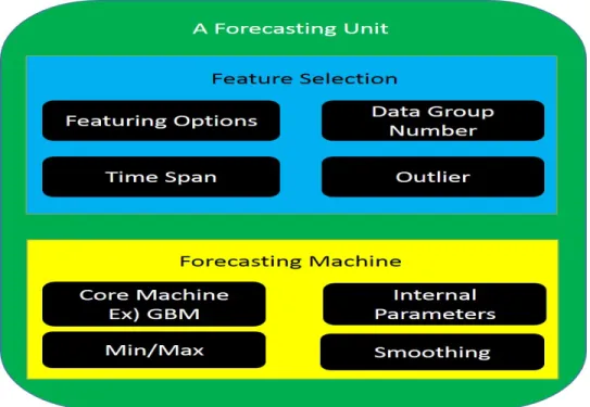
In this chapter, a novel probabilistic and ensemble forecasting algorithm is suggested to predict the hourly wind power output and its probabilistic dis-tribution for a month for ten wind farms. The probabilistic disdis-tribution is given as 1% quantiles. Probabilistic wind power forecasting can provide a solution to reduce the risk to system operations [23] and an opportunity to maximize wind farm owners’ profits [154]. Furthermore, ensemble forecast-ing, which combines multiple forecasting machines with different settings [88] or combines the forecasted wind power of multiple numerical weather pre-diction (NWP) scenarios, can increase the forecasting performance [157]. The framework and techniques are verified using data from the 2014 Global Energy Forecasting Competition (GEFCom).
The probabilistic and ensemble forecasting algorithm is implemented in a new framework, which consists of multiple modules so that users can build case-sensitive forecasting machines by selecting modules. The modules include the feature engineering techniques, preprocessing techniques, and var-ious forecasting machines with different simulation settings. The framework will perform the probabilistic forecasting and ensemble forecasting
simultane-ously by sharing the cross validation. For the probabilistic forecasting, two dif-ferent parametric approaches to estimate the error distribution are proposed. It should be noted that approaches to estimate an error distribution can be classified into the non-parametric approach, in which the prior information about the error distribution is not assumed, and the parametric approach, in which the error distribution is assumed to follow distributions in a closed form. In this study, the parametric approach assumes that the error distribution will follow the approximated variance gamma (VG) distribution and generates dif-ferent distributions with respect to difdif-ferent prediction levels. The continuous function of the conditional error distribution without data classification will also be proposed. The performance of the probabilistic forecasting will be measured by the pin-ball loss. For the ensemble forecasting, the weighted av-eraging, in which the weight factors are estimated by using the shared cross validations, is used. A forecasting unit in the ensemble forecasting is a single combination of a forecasting machine, internal parameters, and simulation set-tings as described in Figure 2.1. The seven forecasting machines are used to create heterogeneity and to increase the performance. These machines are the ridge regression, neural networks (NN), support vector machine (SVM), Gaus-sian process (GP), gradient boosting machine (GBM), random forest (RF), and boosted aggregation (BAG). Furthermore, the optimal memory length of wind speed, best forecasting machines, and their internal parameters are also calculated based on the framework. The proposed forecasting framework is verified using the data in the 2014 Global Energy Forecasting Competition
Figure 2.1: The forecasting unit consists of simulation settings, internal parameters, and forecasting machine.
(GEFCom). The best weekly ranking was second place, and the intermediate ranking was sixth among 215 participants.
2.1
Introduction
Much of the literature has provided non-parametric and parametric approaches to estimate the error distribution of wind power. Many algorithms of the ensemble forecasting have also been proposed.
2.1.1 Literature Review
To increase the performance of wind power forecasting, probabilistic and ensemble forecasting techniques have been researched for a long time. The error distribution of the wind power predictions can be estimated directly from the training data without estimating the wind power predictions by using the special structure of a forecasting machine. For example, in [106], the neural network (NN) is used to generate the prediction interval by building two-output network since one of advantages of the NN compared to other forecasting machines is to have multiple outputs simultaneously. The first output estimates the upper boundary of the given training case, and the second output estimates the lower boundary of the given training case. Weights are updated in order to minimize a special cost function, which tries to increase the probability that the prediction is inside boundaries and to decrease the width of the error distribution. Since this algorithm is only possible within the NN, it cannot use other forecasting machines having high forecasting power. Therefore, it would be beneficial to develop an algorithm to use an ensemble of multiple forecasting machines having high forecasting power compared to the NN. Furthermore, instead of estimating quantiles by stacking lower and upper boundaries, the error distribution can be globally estimated while saving computation time.
Furthermore, instead of changing the internal parameters, in [99], the error distribution is generated by changing the input wind speed. Many differ-ent wind scenarios are generated by putting random noises, which are
gener-ated by using the Monte Carlo simulation, into the vector autoregressive mov-ing average-generalized autoregressive conditional heteroscedastic (VARMA-GARCH) model of wind speed and direction. The error distribution of wind power is estimated by converting many different wind speed scenarios to wind power scenarios using the stochastic power curve, which is based on the condi-tional kernel density. However, this approach might provide the general error distribution, but it cannot provide the tailored distribution with respect to the point forecast and explanatory variables.
Without assuming the parametric or non-parametric error distribu-tions, the quantile can be estimated directly from the explanatory variables. The quantile regression can be used to estimate the error distribution [142]. In this application, developing separate models for each quantile takes a high computation time. Furthermore, better forecasting machines than the regres-sion can be used to estimate the error distribution. The error distribution can also be determined by solving an optimization problem as described in [196]. For example, a direct optimization of both the coverage probability and sharp-ness is used to estimate the optimal error distribution with respect to the performance measure unit of the probabilistic forecasting.
The error distribution can also be estimated independent of forecasting machines. In [156], the adaptive re-sampling method is used to estimate the error distribution based on the classification of wind power without prior infor-mation about the error distribution. On the contrary, instead of re-sampling, it would be advantageous to get the distribution of the forecast errors through
the cross validation. However, the data clustering is also used in this applica-tion in a limited way. For the given predicapplica-tion, its error distribuapplica-tion is trun-cated by the minimum and maximum of the actual values in the prediction’s corresponding cluster. In this paper, an algorithm to estimate the continu-ous function of the conditional error distribution without data classification is proposed. Furthermore, it has already been shown that ensemble forecast-ing can have better forecastforecast-ing power [119], but the forecastforecast-ing power can be further increased by combining tree-based advanced forecasting machines, such as the random forest (RF), bootstrapped aggregation (BAG), and gradi-ent boosted machine (GBM), with differgradi-ent simulation settings. Therefore, as shown in [157], combining probabilistic forecasting and ensemble forecasting might increase the performance of wind power forecasting.
2.1.2 Global Energy Forecasting Competition
As the training data, four explanatory variables, which are the zonal and meridional values of wind speed at 10m and 100m, are provided for 10 wind farms, so there are 40 explanatory variables. The error distribution of one-hour-ahead wind power outputs were forecasted for ten wind farms. The x-axis and y-axis values of wind speed at 10m and 100m were provided. Wind speed was also predicted based on one-hour-ahead NWP. The error distribution was represented as 99 quantiles. This competition consists of 15 competitions for 15 weeks. Every week, one hour-ahead wind power for a month was forecasted. In the next week, wind power for the next month was
forecasted, and the testing data in this week became the last month of the training data in the next week. In this study, the data from the only second week is used. The training data was measured from 1/1/2012 to 10/31/2012, and the testing part is from November, 2012.
2.2
Program Architecture
In this section, the architecture of the forecasting program is intro-duced. In a broad sense, the forecasting program consists of three stages. The first and second stages share the same internal forecasting process with the same simulation settings.
2.2.1 External Forecasting Process
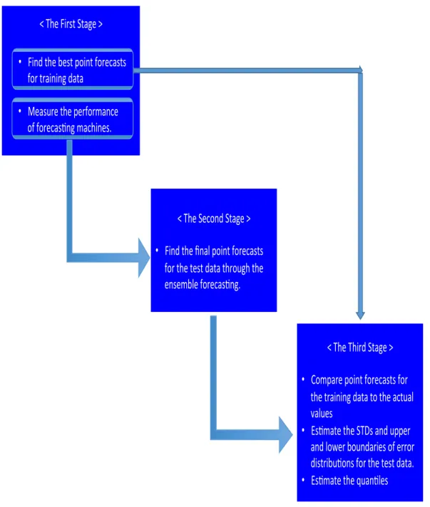
In the first stage, the performances of forecasting units are measured using the root mean square error (RMSE) through the external five-fold cross validation where the training data is classified into the actual training data and validation data. In this application, 20% of the data is selected as vali-dation data recursively. Furthermore, point forecasts for the valivali-dation data are estimated through the ensemble forecasting. In the second stage, the final point forecasts for the test data are estimated through the weighted ensemble forecasting, in which weight factors are set as inversely proportional to the forecasting machines’ RMSEs, which are estimated in the first stage. In the third stage, the standard deviations (STD) of the error distribution of the test data are estimated by comparing the point forecasts for the validation data in
the first stage to their actual values. The step-wise process of three stages is shown in Figure. 2.2.
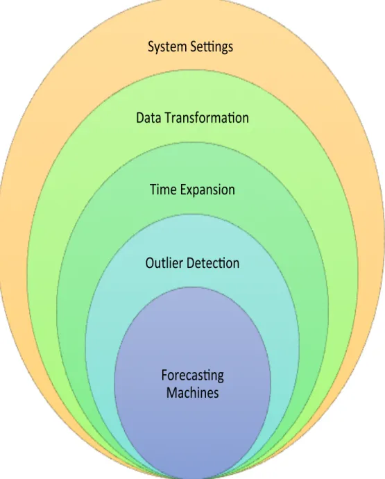
2.2.2 Internal Forecasting
As mentioned above, the wind power is actually forecasted by the fore-casting units in the second and third stages. The forefore-casting units in both stages are built according to the same various layers of simulation settings, which is described in Figure 2.4. Many combinations of different simulation settings can be structured in a tree, and the tree structure is implemented in this program through five for-loops that are layered. Since each loop has multiple options, the total number of simulations is the multiplication of the number of options in each layer. The five layers consist of system parameter settings, data transformation, time expansion, outlier detection, and individ-ual forecasting machines. The structure is shown in Figure 2.3. In the first sequence, different fixed parameters of forecasting machines are set. Then, the training data is expanded by adding the quadratic, cubic, and square of root terms in order to extract the nonlinear relationship between wind speed and wind power. Furthermore, the wind speed on the target day is expanded by adding new features that include time information and forecasted weather data on the day before and the day after the target day. Outliers are also defined and removed. In the preprocessing, each feature of each class has a zero mean and uniform standard deviation (STD). For the given actual training data, the internal cross validation is used to determine the optimal parameters in the
< The First Stage >
< The Second Stage >
•
Find the final point forecasts
for the test data through the
ensemble forecas:ng.
< The Third Stage >
•
Compare point forecasts for
the training data to the actual
values
•
Es:mate the STDs and upper
and lower boundaries of error
distribu:ons for the test data.
•
Es:mate the quan:les
•
Find the best point forecasts
for training data
•
Measure the performance
of forecas:ng machines.
Figure 2.2: The three-stage program architecture is introduced. The best forecast-ing units, STDs, minimum, and maximum of quantile for each output groups are delivered from the first stage to the second stage.
forecasting machines. Twenty percent of the training data is set aside to verify the internal parameters. Finally, the predictions are smoothed, the minimum level of predictions is limited to zero, and the maximum level of predictions is limited to the maximum value of training data.
2.2.3 First Stage
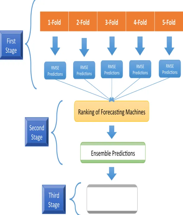
In the first stage, point forecasts for the training data and the perfor-mance of the forecasting units are estimated. The external five-fold cross val-idation is used to measure the performance of the forecasting units. However, in the internal cross validation, when the internal parameters of forecasting machines are estimated, different validation data is selected from the actual training data to select the optimal internal parameters of forecasting machines. The point forecasts for the training data are generated through the ensemble forecasting using the predictions of forecasting units. The strategy with en-semble forecasting is to make as many different input or feature matrices as possible and run them with different forecasting machines.
Since all forecasting units are evaluated through the same validation data, the performances are compared fairly. Furthermore, since the validation set is alternatively built through the external five-fold cross validation, the point forecasts for all training data can be estimated. Then, the point fore-casts of training data are estimated by averaging the predictions of forecasting units with weight factors. Therefore, in the first stage, the performances of the forecasting units are estimated and used to estimate the point forecasts
System Se(ngs
Data Transforma1on
Time Expansion
Outlier Detec1on
Forecas1ng
Machines
1-‐Fold
2-‐Fold
3-‐Fold
4-‐Fold
5-‐Fold
RMSE
Predic,ons Predic,ons RMSE
RMSE
Predic,ons Predic,ons RMSE
RMSE Predic,ons
Ranking of Forecas,ng Machines
Ensemble Predic,ons
Error Distribu,on
(STD, Min, Max)
First
Stage
Second
Stage
Third
Stage
for the training data. The performances are also used to estimate the point forecasts for the test data in the second stage. In addition, in the third stage, point forecasts for all training data are used to estimate the STDs of error dis-tributions, lower boundaries, and upper boundaries by comparing them with the actual values.
2.2.4 Second Stage
In the second stage, all training data is considered as the actual training data, and the final point forecasts for the test data are estimated through the ensemble forecasting by using the RMSEs in the first stage. In other words, forecasting units are re-trained using all training data. If the number of forecasting units is high, or if the performances of a few forecasting units are much lower than those of other forecasting units, a few best combinations in the first stage are used in the second stage. It should be noted that the computation time of the second stage is less than that of the first stage since it does not need to perform the external cross validation.
2.2.5 Third Stage
The point forecast of validation data are compared to the actual vali-dation data in order to estimate the standard deviation, maximum, and min-imum values of the error distribution under the assumption that the error distribution follows the approximated VG distribution. In the non-parametric approach with the data classification, the point forecast in a different group
is compared to the validation data in the same group, and each group has different standard deviation, maximum, and minimum values of the error dis-tribution. The optimal STD is determined when a candidate STD minimizes the sum of the quantile errors of the point forecasts in each group. By increas-ing the STD from zero, the sum of measured quantile errors is calculated with respect to the STDs. On the contrary, in the non-parametric approach with-out the data classification, the optimal STDs of each point forecast of the test case is estimated with respect to the point forecast of the test data through another forecasting machine. In order to train this forecasting machine, the optimal STDs of the training data are used as the target data, and the weather data and point forecasts of the training data are used as training data for this forecasting machine. In short, this forecasting machine calculates the opti-mal STDs as a function of weather data and point forecasts. However, in the non-parametric approach, the data classification is also used to determine the maximum and minimum values of the error distributions. Therefore, for the given point forecast of the test data, the minimum and maximum values of wind power in the cluster that the point forecast belongs to are used to limit the error distribution of that point forecast.
2.3
Feature Engineering
The goal of feature engineering is to design the number of rows and columns of the input data matrix to generate the training data. In this section, feature engineering methods to tailor the input data matrix are explained
AMP10 AMP10 2 AMP10 3 AMP100 AMP100 2 AMP100 3 Correlation Coefficient 0.6 0.65 0.7 0.75
0.8 Correlation Coefficients Analysis
Figure 2.5: Correlation coefficients of transformed amplitudes of wind speed at 10m and 100m are plotted. The linear, quadratic, and cubic of amplitudes of wind speed at 10m and 100m are shown respectively.
individually.
2.3.1 Data Smoothing
The absolute value of raw wind speed data is smoothed in order to rep-resent the dynamic movement of wind speed since NWP data that is generally sampled at a fixed interval cannot represent the time series characteristics of wind speed. In the competition, the moving average is used, and the optimal length of the moving window per wind farm is also decided.
2.3.2 Data Transformation
The input features are transformed into the quadratic and cubic in or-der to extract the nonlinear relationship between wind speed and wind power. The transformed input features include the zonal component, meridional com-ponent, and amplitude of wind speed at 10m and 100m. For example, the correlations of amplitudes of wind speed at 10m and 100m are compared to the correlations of the squared amplitudes and cubic amplitudes in Figure 2.5. It is observed that the wind speed at 100m is more highly correlated than the wind speed at 10m, although it is widely known that the cubic of wind speed is more highly correlated than the linear wind speed. It should be noted that the interaction terms of multiplication among features are not consid-ered since including the interaction terms increases the number of variables exponentially.
2.3.3 Data Expansion
Since wind speed at any given moment is highly correlated with the wind speed an hour before and an hour after the given moment, in order to consider the dynamic nature of wind speed, all predictors from t−k to t+k are used to predict wind power at t. This data expansion technique can also control the number of variables, so it can also control over-fitting. The length of the timespan could differ based on the training data, but generally k is set at one or two. However, a three-hour timespan deteriorates the forecasting performance. In the ensemble forecasting, different timespans are used for
multiple forecasting units, and a few best forecasting units are selected. Fur-thermore, month, day, days of the year from one to 365, and year are added in order to extract the seasonal trends.
2.3.4 Outlier Detection
Outliers are defined and removed from the feature space. Predictors are ranked according to the difference between the target value and the prediction value forecasted by the ridge regression. The errors are measured as the abso-lute of this difference, and errors are sorted in descending order. It should be noted that each wind farm has its own outliers. Furthermore, the fraction be-tween the outliers and training data should be searched before the simulation. The top 5% of errors are generally defined as outliers and removed. It is also interesting to observe that every forecasting machine has a different ability to resist outliers. For example, the NN seems to be weak for outliers, but the SVM is resistant to outliers. Furthermore, it is known that the GBM and RF are typically resistant to outliers [97], but they are susceptible to outliers in this simulation.
2.3.5 Input Data Classification
Wind power data can be classified into three groups with respect to the amplitude of wind speed. Generally, the power curve of the wind turbine can be classified into three ranges: wind speed less than the cut-in speed, wind speed between the cut-in speed and cut-out speed, and wind speed more
than the cut-out speed. However, since the performance of a single group is better than that of three groups, the input data classification is not used in this application.
2.3.6 Pre-processing and Post-processing
After the simulations, 18 variables have shown the best performance. They are the zonal component of wind speed at 10m, zonal component of wind speed at 100m, meridional component of wind speed at 10m, meridional com-ponent of wind speed at 100m, amplitude of wind speed at 10m, amplitude of wind speed at 100m, square of zonal component at 10m, square of zonal com-ponent at 100m, square of meridional comcom-ponent at 10m, square of meridional component at 100m, cubic of meridional component at 10m, cubic of merid-ional component at 100m, square of amplitude at 10m, square of amplitude at 100m, cubic of amplitude at 10m, cubic of amplitude at 100m, angle of the cylindrical coordinate of wind speed at 10m, and angle of the cylindrical coordinate of wind speed at 100m. If predictors in the previous hour and next hour are included, the number of variables increases to 54. Then, predictions from ten wind farms are aggregated, so the number of variables increases to 544 by including day, month, day of the year, and year. However, since some features are shared between wind farms, the final number of variables is 528.
However, according to the input data generation method, the number of total features is changed. Therefore, many options are offered to control the number of features. For example, the first input data option has only raw
observation data, the second input data option has linear and quadratic terms of input data, and options become more complex after that.
Then, training data has a zero mean and has one as the standard de-viation before it enters into the forecasting machines. After wind power is forecasted, the final prediction is smoothed. In addition, the prediction per wind farm is limited by the minimum and the maximum of each wind farm. 2.3.7 Simulation Settings for Individual Forecasting Machines
Different simulation settings are fixed before running the forecasting. Simulation settings include the ratio of the number of outliers, the outlier detecting machine, and some fixed internal parameters in forecasting machines. Some simulation settings that can outperform other settings are set before the training data enters the loops in order to increase the system efficiency. Therefore, if the best settings are detected, they are enumerated in the code. It should be noted that the prediction horizon is not considered, and the ensembles of NWP with different initial settings are not used in this case study. If the prediction horizon needs to be considered, it would be preferably to have different forecasting machines for each prediction horizon.
2.4
Forecasting Machines
In this section, seven forecasting machines are introduced: ridge re-gression, NN, SVM, GP, GBM, RF, and BAG. The forecasting machines used in this study can be classified into regression models, kernel-based models,