Nurikabi Solver

(1)

NURIKABI SOLVER

Deepika Dasari Soorasamharan, Pranamita Nanda

Velammal Institute of Technology, Panchetti, Tiruvallur District, Tamilnadu, India

ABSTRACT

Nurikabe is logical puzzle game. Nurikabe puzzle normally has „m‟ number of rows and „n‟ number of columns. Even though it is a logical puzzle game, one cannot solve all the puzzles with pure set of logics. Because Nurikabe puzzle is a NP-complete game. Hence some assumptions must be made in order to solve the given puzzle. In this project in order to make this kind of assumptions with set of logics, SAT solver is used. SAT solver is an efficient tool to make the decisions with binary logics. SAT solver will accept only CNF format. So the puzzle rules and solving logics are converted into CNF format and given to SAT solver. Results from the SAT solver are checked with the rules and if the result satisfies the rules, then it is determined that the result as an appropriate solution for the given puzzle. And new Nurikabe puzzles also generated within certain limit in this project. SAT solver is used to generate new puzzles in this project.

Keywords: NP-complete, Conjunctive Normal Form, T Veerarajan, Nurikabe puzzles

I. INTRODUCTION

Nurikabe is a binary determination puzzle game, published by Nikoli. Nurikabe consists of M*N grid that is it has m number of rows and n number of columns. Nurikabe is a Japanese word which means that invisible wall that delays the path. Users have to follow set of rules to find the hidden wall. To solve the puzzles automatically, SAT solver tool will be used. Sample Nurikabe games are available online [1].

More logics and strategies have to be followed in order to computerize the puzzle game. The rules to play the Nurikabe puzzle is described as follows,

 Cells are considered to be connected only if it is connected either vertically or horizontally.

 Each numbered white cells should have the

same number of white cells around it.

 All the black cells should be connected and the

grid should not have any 2x2 black pools.

A. Motivation

Puzzle games are getting more popular day by day. While implementing the puzzle game in software it

requires more logics and strategies to obtain the solution and it can be helpful to increase the ability to create new logics for any given problem. SAT solver is a tool which is popular in solving satisfiability problems [3]. SAT solver tools are open-source, available under free license and it has vast implementations. SAT solver is a powerful tool in decision making, software verification and it is used in artificial intelligence. Instances for SAT solvers are miniSAT, SAT4j, GRASP, PicoSAT, HyperSAT, RSAT and so on. SAT solvers are available for C, C++, JAVA, C# platforms and all SAT solvers are available online for free downloads [2]. And it can be implemented with Formal Languages such as Z- Language. SAT solvers are flexible and it can be modified.

B. Aim

The aim of the project is to computerize the Nurikabe puzzle and to implement the automatic solving functionality and to implement the generating new puzzles functionality.

C. Objective

(2)

filled with black and white colours according to the given numbers in the puzzle game. White cells are known as path or Islands and connected black cells are known as walls or streams. Initially wall is invisible and after solving the puzzle with the rules, connected wall will be revealed. Puzzle matrix will be converted into SAT instances and it will be given to the SAT solver. SAT solver will solve SAT instances with the help of puzzle logics given to it. And outcome of the SAT solver will be displayed as a result. Firstly Graphical User Interface (GUI) has to be created to display the puzzle as well as to play the puzzle. Secondly puzzle logic for Nurikabe puzzle game should be created and it should be implemented with the SAT solver. Thirdly, checking for the user input and verifying the solution given by the user has to be done and finally solving the entire puzzle automatically and showing the result to the user with the help of Graphical user interface.

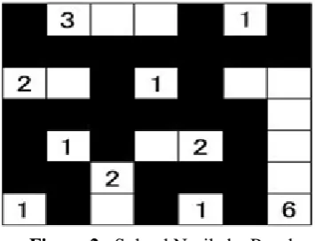
Figure 1 : Unsolved Nurikabe Puzzle

Figure 2 : Solved Nurikabe Puzzle

D. Literature Review

1. Ines Lynce, Joel Ouaknine Sudoku as a SAT

Problem

This paper holds the vital clue for how the puzzle logic can be converted to the propositional logic. Also we can understand how the CNF (Conjunctive Normal Form) can be generated out of the propositional logics and

encoding techniques for the SAT solver.

2. Daniel Le Berre: From SAT to SAT4J

This paper describes the uses of SAT solvers and its advantages and which format of the input is needed for SAT4J. It describes about how to derive the CNF from the Propositional formula. And it tells how the SAT4J can be integrated with the Java platform. From this paper we can understand efficiency of the SAT solver. This paper is used to understand about the basics of SAT solvers and CNF formats.

3. T Veerarajan: Discrete mathematics (Chapter 1: Mathematical logic)

First chapter of this book is used to understand the Normal forms and its principals, conversion of one form to the other (DNF to CNF), Laws of Algebra of propositions which includes De-Morgan‟s Law. And it provides many examples for all those things mentioned above.

II. METHODS AND MATERIAL

1. Technical specification

The Nurikabe solver is developed with:

 NetBeans IDE 7.0

 JAVA - jdk 1.6

 SAT solver – SAT4J

A. NetBeans IDE 7.0

NetBeans is an open source IDE which will support many languages like java, C, C++, PHP and so on. In this project java swing technologies are used which can support JButton, JFrame, JMenu, JMenuBar etc. More than that Java swing is very simple to implement compared to the Java applets. But NetBeans IDE needs Java Development Kit to run the java projects. For this project JDK 1.6 is used. Both NetBeans and JDK is available for free of cost.

B. Project Analysis and Design

(3)

design in a significant manner. GUI is developed using the Net Beans IDE 7.0, jdk 1.6 and SAT4j library. SAT4j has many kinds of library files. In this project, core library file of the SAT4j is used. This core library file is easy to implement any we can easily work with its functionalities. All kind of implementation methods are available in the SAT4j documentation [8]. Predefined puzzle questions are stored in separate text file. Inside that text file every data is given such as the row size and column size and followed by the numbers to display in the grid. To represent the empty cell in any coordinate in the puzzle grid we should enter the number „0‟ in the appropriate coordinate of the question text-file. Example for this text file is shown in the following diagram,

Figure 3 : Text file which shows format of the puzzle question

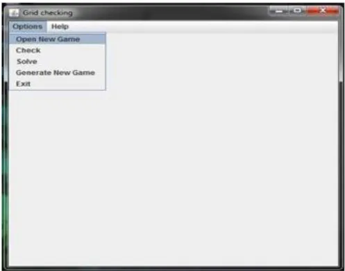
While loading the new game, number of rows and number of columns will be obtained to define the size of the grid and to define the number of rows and columns in the grid. All the functionalities such as “Open new game”, “Check”, “Solve”, “Generate new game” and “Exit” are added to the “Options” menu and “Rules” functionality is added to the “Help” menu.

The functionality “Open new game” will go to the “List of games” folder as per the address given to it. After locating the “List of games” folder, this functionality will start to count the number of files available inside that folder. That number of files is used as a maximum limit. If user clicks the “Open new game” functionality for the first time then first file inside the “List of games” folder will be selected first. If the user clicks the “Open new game” functionality for the nth

time, then nth file in the “List of games” folder will be selected. If number of clicks exceeds the maximum limit of the count of number of files available inside that “List of games” folder, then the number of clicks is assigned to zero. So when the number of clicks exceeds the maximum limit of the number of files available, then first file from that “List of games” folder will be selected next. This functionality will count the number of files available in the “List of games” folder each time the user clicks this

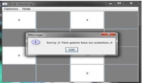
functionality. So it is possible to introduce the new game file during the run time of this project. If any of the game file is not having sufficient numbers or not created in the specific format, then it will not load the game and it will show the message box to the user, which holds the message like “Sorry..!! Could not load this game”. The image showing this message box is given below,

Figure 4 : Message box showing the inconvenience in loading the game

If the selected file is in the correct format then the selected game will be displayed in the main window grid. Initially all the cells in the grid will be grey in colour except the numbered cells.

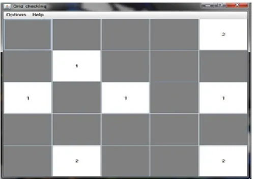
All the numbered cells will be white in colour. Grey coloured cells are unknown cells. If the grey cell is clicked once it will change its colour to white. If the white cells are clicked once, then it will change to black in colour and if any black cell is clicked then it will change to white in colour. Any colour change will not happen to the numbered cells and it will be white in colour for ever. The “open new game” functionality is displayed in the image below.

(4)

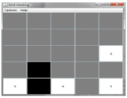
Figure 6 : Sample Nurikabe Puzzle game

The “Check” functionality will check for the correctness of the user solution. In this check functionality four check points are implemented. First check point will check for the number of black cells and white cells. If we subtract the sum of the numbers from all the numbered white cells from the total number of cells then we can find the number of actual black cells.

Number of Actual black cells = Total number of cells – Sum of numbers in numbered white cells.

If the count of black cells is same as the actual black cells which we got from the above formula then first check point will return true. If not then it will return false.

Second check point will look for the 2x2 black pools in the grid area. In the M*N grid it is enough to run the loop till (m-1)x(n-1). Because if we start form the first cell which has the coordinate of (m=1, n=1), then this check point will look for its neighbours colour which are having the coordinates (m=1, n=2), (m=2, n=1) and (m=2, n=2). By the moment the loop reaches the coordinate (m-1, n-1), this check point would have processed all the cells in the grid. If there are no 2x2 black pools formed then the second check point will return true. If not it will return false.

Third check point is developed to check for the continuity of the black cells and it will find the isolated black cells also. For the convenient the solution provided by the user will be converted to the matrix form which will have only 0s and 1s. 0s will represent the white cells and 1s will represent the black cells. To find the continuity of the black cells DFS (Depth first

search) algorithm is used. DFS is very efficient in finding the depth of the given tree. And DFS is very efficient in finding the path in Maze puzzle games [5][10]. This Depth first algorithm is configured to traverse along the black cells and to count the number of black cells that are present in its way. And also it is configured to look for the isolated black cells in the grid. To traverse along the black cells recursive form of the DFS is used. So it will call itself again and again till it reaches the end. This third check point will return true if it is not finding any isolated black cells and the counting of the black cells is same as the actual black cells. Otherwise it will return false. Actual number of black cells is the difference between the total size of the grid to the counting of the all the numbers in the numbered cells available in the grid.

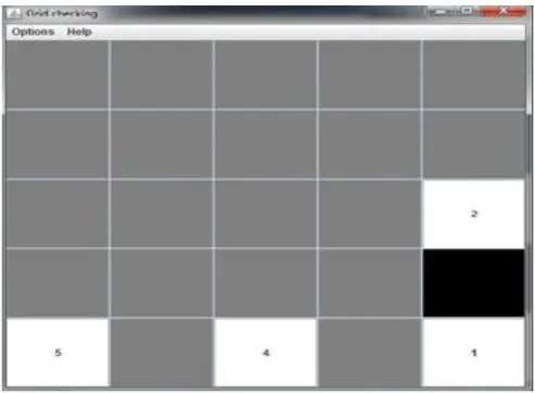
Coordinates to the algorithm is the first occurrence of the black cell in the whole grid. All the cells inside grid are converted into 0s and 1s and it is stored in the array. Number 0 represents white cells and Number 1 represents black cells in the grid. This algorithm can be explained with the following images,

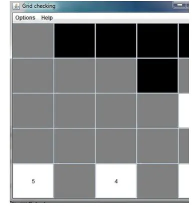
Figure 7 : Sample Nurikabe Puzzle game with partial solution

First the above grid is converted to the matrix form as mentioned above. The matrix for the above grid is shown below.

1 1 0 1 0 1 0 1 1 0 0 1

(5)

coordinates firstly in the segment 1. The coordinates are safe to process, because they are inside the matrix. And it will check for the acknowledgements whether this is processed before or not in the segment 2. In this case it was not acknowledged before. So it will go to the next step of the process which is segment 3. Segment 3 is to check whether the count of the number of black cells reached the number of actual black cells or not. In this case it has not reached yet. So it will go to the next step which is segment 4. Here it will check whether the cell which is in process, is black or not. If it is black then it will allow going to the next step. If not, then it will return false to the function. In this case it is a black cell, so it will not return false and it will go to the next step. In the segment 5, if the current coordinates has black cell then it will acknowledge that the current cell is processed and it will increase its variable named „pathcount‟ by 1 and it will check for its neighbours. Here the function is called with the same set of matrix with the neighbour coordinates. In this example only two cells are connected to the cell with the (m=1, n=1). So the „pathcount‟ value will be 3. Because, other black cells have no connection either vertically or horizontally with the first black cell. If any of the black cells has no neighbour, then it will be marked as the isolated cell. In this example, expected number of connected black cells (path-count) is 8 which is the count of the actual black cells. But only 3 connected black cells are found from the first cell. So it does not satisfy the rules. Hence check3 will be assigned as false in this example. If we consider the following diagram,

Figure 8 : Sample Nurikabe Puzzle game with full solution

This example diagram satisfies the check point 3. Because in the above example, number of cells is 12. And the actual number of black cells is 8 and the count

of the current black cells is also 8. So this check point 3 will return true in this case.

Fourth check point is developed to check for the number of white cells connected to the numbered white cells. This fourth check point is also based on DFS algorithm [5][10]. DFS algorithm is configured to find the numbered white cells and the connected white cells to it. It is configured to traverse only along the white cells. This check point will return true if the numbered white cells in the grid has the same number of white cells around it. If it detects any numbered white cells that have more number of white cells around it or less number of white cells around it, then it will return false.

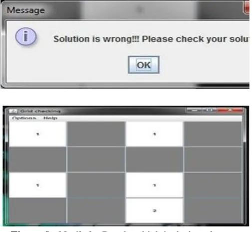
If all these four check points returns true then the solution is correct and it has no error in it. And it will show the confirmation message of the correctness. If any of the checkpoint fails and returns false then it will show the failure notification in the message dialogue and the message dialogue is shown below.

(6)

Figure 10 : Message dialogue which shows failure notification of the given puzzle

To check the accuracy of the solutions during each iteration, DFS algorithm is used. Here also DFS is modified in two ways as same as the checking functionality. One is to find the number of connected black cells and the other DFS is modified to look for the number of white cells around the numbered white cells. To increase the efficiency of the checking process some tactics are followed. When the SAT solver returns the “satisfiable” answer, accuracy of that solution has to be checked. Before doing the checking for the number of connected white cells with modified-DFS algorithm, accuracy in the actual number of white cells with the current number of white is checked. To do this process, while extracting the answer given by the SAT solver to do the appending operation, number of white cells available in that solution is calculated. If the calculated number of white cells is same as the sum of numbered cells available in the grid, then it will allow the solution for the further checking. If not it will not go further and it give the inverted solution to append to get the next possible solution. If the actual number of white cells is same as the current number of white cells, then the checking for the number of connected black cells will be done. If checking for those black cells returns false at any moment, then it will terminate the current process and the current solution will be inverted and appended to the CNF file. If it returns true, then the checking for the number of white cells around the numbered white cells will be done. If any of the numbered cells has low or high number of white cells around it compared to the number inside the numbered cell, then it will return false and it will allow the inverting and appending process of the current solution to the CNF file. If all of the above checking returns true, then the current possible solution is the exact solution which obeys all of the Nurikabe rules. And it will show the message dialogue which has

the message like “Congratulations..!! You have finished the game..!!”. The diagram showing this message dialogue is as follows.

The functionality called “Generate New Game” is used to generate new games which are of 5x5 in size. To generate the new game, one important rule is taken firstly. That is no 2x2 pool formation inside the grid. This rule to avoid the 2x2 pool inside the grid is written inside the CNF file named “gen.cnf”. After that whole “gen.cnf” file will be replaced to the “generate.cnf” file in correct format. Random number is generated within the limit. Many methods are available to generate the random numbers within the limit [11]. In this project, random number is generated which is within the range from 1 to 100. Till that generated number loop will run and inside that “generate.cnf” will be red and its solution will be updated to the “gen.cnf” and this process will continue till the loop reaches the generated number. After this process all the black cells inside the grid will be converted into number 1 and white cells inside it will be converted into number 0 and it will be stored in the matrix. This stored matrix and the coordinated of the first black cells in the grid is given to the modified-DFS

algorithm named „pathtracking_gen‟. This

(7)

„matrix‟. This can be explained with the following example.

„martix‟ 0 0 0 0 1 1 1 1 1 1 1 0 0 0 1 1 0 0 1 1 1 1 1 1 0

In this example „pathtracking_gen‟ will return true. Because number of black cells in the above matrix is 15. And number of continuous black cells in the region also 15. So it will return true value. So it will go for the „check_boundedness_gen‟ algorithm as a next step.

Here first occurrence of the white cell (Number 0) is in

the coordinates (m=1,n=1). After calling

„check_boundedness_gen‟ algorithm we will get the „A-matrix‟ as follows,

„A-matrix‟ 4 0 0 0 0 0 0 0 0 0 0 0 0 0 0 0 0 0 0 0 0 0 0 0 0

And the „check_boundedness_gen‟ algorithm will start from the second occurrence of the „matrix‟ which has the coordinates (m=1, n=2). But the count of the white cells will be 0 this time. Because this second occurrence of white cell with coordinates (m=1. n=2) is already processed. So the number of continuous white cells will

be 0. After the completion of this

„check_boundedness_gen‟ for the entire matrix, we will get the „A-matrix‟ as follows,

„A-matrix‟ 4 0 0 0 0 0 0 0 0 0 0 5 0 0 0 0 0 0 0 0 0 0 0 0 1

This „A-matrix‟ is used to display the questions in the grid. And the „matrix‟ will be used to check for the user‟s solution as well as to display the correct solution, when the user is calling „solve‟ function.

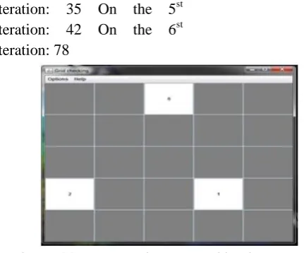
On the 1st iteration: 65 On the 2st iteration: 95 On the 3st iteration: 77 On the 4st

iteration: 35 On the 5st iteration: 42 On the 6st iteration: 78

Figure 11: New puzzle generated by the “Generate New Puzzle” functionality

In this example, the first 5 random numbers are failed to provide the continuous black cells without any isolated black cells. And in the 6th iteration the random number 78 is generated and it has provided the continuous black cells.

The functionality called “exit” is to close the Nurikabe puzzle game tool.

And the help functionality is implemented to display the message box which will display the set of rules to be followed in order to play the Nurikabe puzzle game. This message box is showed in the following picture.

Figure 12: Message dialogue shows the rules

III. RESULTS AND DISCUSSION

Project Development

A. Logic formula

(8)

whether the given problem is satisfiable or not.

For the formation of propositional logic formula, the following symbols will be used commonly.

→ Then ⌐ Negation

AND (or) Conjunction OR (or) Disjunction ↔ Same as

Deep understanding of the game has provided many clues to solve the given game with SAT solver. SAT solver will accept only Boolean forms. So eventually we are converting entire game and its solving steps into the Boolean format which consists of only true and false. Nurikabe has only Black and White cells in its solution and those white and black cells have to be filled with logic. Some assumptions are made to solve the game. The first assumption is TRUE indicates white cell and FALSE indicates black cell. And the Second assumption is if the cell has number in it then that cell must be white.

Sample logic formula is given below,

S (m, n)=1 → S(m-1, n)=false _ S(m+1, n)=false _ S(m,

n+1)=false _ S(m, n-1) =false

This formula represents the simple solving logic in the Nurikabe puzzle game. It means that if the cell which has the coordinates of row=4 and column=4 has the number 1 and it is white in colour, then the cells around it with coordinates (3,4), (5,4), (4,5) and (4,3) will be converted into black. The formula given above is in DNF (Disjunctive normal form) format. SAT solver will accept only CNF format. So the formula can be written as follows,

S(m, n)=1 → S(m-1, n)=false S(m, n)=1 → S(m+1, n)=false S(m, n)=1 → S(m, n+1)=false S(m, n)=1 → S(m, n-1) =false

If number 2 is found in any cell in the game then the logic to solve that will be as follows,

S(m, n)=2 → S(m, n)=true _ (S(m-1, n)=true S(m+1, n)= true _ S(m, n+1)= true _ S(m, n-1) = true)

This formula describes that if the number 2 is found in the 2nd row of the 2nd column then that cell must be true and any one of the cells around it (1st row of the 2nd column OR 3rd row of the 2nd column OR 2nd row of the 1st column OR 2nd row of the 3rd column) must be true. So in the CNF format it can be written as follows,

S22=2 → S22=true

S22=2 → S12=true _ S32=true _ S21=true _

S23=true

This S22=2 → S12=true _ S32=true _ S21=true _

S23=true condition will give at-least 1 true variable at

a time. So it means that it can give more than 1 true variable at a time. Other combinations except 1 true variable at a time are as follows,

Total Number of Number of

number of True combinations

variables variables at available

(X )

a time

( C =X! / (

X-( T ) T)! T! )

4 2 6

4 3 4

4 4 1

So total remaining combinations are (6+4+1) = 11

These combinations are unnecessary and it increases the number of iteration to find the exact solution. So we have to avoid those combinations. To avoid those combinations, only way is to get those combinations and if we invert those combinations and if we append it to the CNF file, we can get the results, which are all having only 1 true variables at a time. So the resulting combination will be only 4 combinations in which only one true variable available at time.

If we consider the following condition, B _ C _ D

(9)

where T= True and F= False,

B C D B _ Satisfiability

C _ D

T T T T Satisfied

T T F T Satisfied

T F T T Satisfied

T F F T Satisfied

F T T T Satisfied

F T F T Satisfied

F F T T Satisfied

F F F F Unsatisfied

If we consider three variables B, C and D with the following combination,

(B _ C) _ (C _ D) _ (B _ D)

It will give at least 2 true variables at a time. In the above combination 1 variable is skipped at a time. In order to attain at least 2 true variables at a time from three variables, three different combinations are needed with 1 variable skipped in each combination.

If we consider „X‟ variables with 2 variables skipped at a time in its combination, then it will give at least 3 true variables at a time.

If we consider „X‟ number of variables with „S‟ number of variables skipped at a time then the combination will give at least „S+1‟ true variables at a time.

The following table describes the relationship between skipped number of variables and minimum number of true variables.

Number Skipped Minimu Maximu

of number m m

Variable of number number

s variable of true of true

( X )

s values values

( S ) ( Min = ( Max = X

S+1 ) )

10 1 2 10

10 2 3 10

10 3 4 10

10 4 5 10

10 5 6 10

If number 3 is found in the coordinate (m, n) then the possible region cells will be,

S(m-1, n), S(m-2, n), S(m+1, n), S(m+2, n), S(m, n+1), S(m, n+2), S(m, n-2), S(m, n-1), S(m+1, n-1), S(m-1, n+1), S(m-1, n-1), S(m+1, n+1)

We know that numbered cell must be white. To complete its region, 2 more cells are needed. So we have to skip 1 variable at a time in its possible region cells to obtain the correct combination.

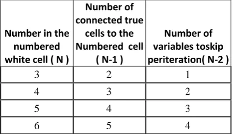
Therefore if the number „N‟ is found in the Nurikabe grid then, N-1 cells around it must be true and those cells must be connected either horizontally or

vertically. The number of variables to skip will be N-2 for the formation of its possible region. The following table describes the relationship between the number and the number of variables to skip per iteration and the number of true cells.

Number in the numbered white cell ( N )

Number of connected true

cells to the Numbered cell

( N-1 )

Number of variables toskip periteration( N-2 )

3 2 1

4 3 2

5 4 3

6 5 4

From the complete understanding of the game, it is possible to determine the possible region of cells. After finding all the set of cells from the possible region, it will be simple to determine the cells from the impossible region. To understand this concept the following diagram can be used.

Figure 13: Showing the Possible region of the

(10)

In the above diagram, green coloured cells are the possible region cells for the cell with number 4. Generally the maximum number of possible region cells for any numbered cells will differ from „N-1‟ to „N2

+ (N-1)2 – 1‟ where N is the number in the numbered cell. Examples for this can be seen in the following table,

Number ( N )

Minimum no. of possible region cells ( N-1 )

Maximum no. of possible region cells ( N2 + (N-1)2 – 1)

2 1 4

3 2 12

4 3 24

5 4 40

6 5 60

An algorithm is developed to determine the possible region cells for the numbered cells. That algorithm is shown below, after finding all the possible region cells, there is a need to create all the possible combinations with the appropriate number of variables skipped. To create the combination of the possible area cells, the following algorithm is developed.

Deep understanding and analysis of the relationship between number of variables and the number of variables to be skipped reveals some structures. This analysis is explained with the help of following table,

Number of possible cells for

any numbered cell ( X )

Number of variables to skip per iteration ( S )

Number of combinations achieved ( C =X! / ( X-S)! S! )

6 1 6

6 2 15

6 3 20

6 4 15

6 5 6

In the above table X! is known as Factorial of X. For example if X = 5 and S = 2, then the total number of possible combinations will be,

C = ( 5! / ( 5 - 2 )! 2! ) = ( 5*4*3*2*1) / (3*2*1)*(2*1) = 10

So in this example total combinations will be 10.

For every numbered cell, its entire possible region is collected and inverted and given to the SAT solver to avoid the all-true condition. Because the formulas and combinations will give at-least conditions only. Example explained with the possible area cells of number 3 is as follows,

S(m-1, n) _-S(m-2, n) _- S(m+1, n) _- S(m+2, n) _- S(m, n+1) _- S(m, n+2) _- S(m, n-2) _- S(m, n-1) _- S(m+1, n-1)- S(m-1, n+1) _- S(m-1, n-1) _- S(m+1, n+1)

At the same time rules also have to be implemented to attain a solution for the given game. It is very hard to implement the rules like boundedness of the numbered white cells and the continuity of the black cells. But it is simple to implement the rule like 2x2 pools is easy in the CNF. Propositional logic to avoid the 2x2 pool of black cells will be as follows,

S(m, n) _ S(m+1, n) _ S(m, n+1) _ S(m+1, n+1)

The above formula clearly states that at least one of the cells in the four cells must be true. But with this propositional formula number of solutions made by the SAT solver will be very high. From that list of solutions we can find the unique answer for the given game. It is not efficient and it will take more time to get the proper solution from the list of solutions. So we tend to create some more propositional tactics to minimize the list of solutions as well as to reduce the time to search for an appropriate solution from the list.

In the Nurikabe matrix if we find any numbered cell then it must be white. So we can convert this logic into propositional logic as follows,

S(m, n) ≥ 1 → S(m, n) =true

And In the Nurikabe matrix if we find any numbered cells that have more than number 2 in it, then one of the cells around it either horizontally or vertically will definitely be true. So the propositional logic for that will be as follows,

S(m, n) ≥ 3 → S(m-1, n)=true _ S(m+1, n)= true _ S(m, n+1)= true _ S (m, n-1) = true

(11)

In the Nurikabe grid if we find any two numbered cells that are diagonally adjacent, then the propositional formula will be as follows,

S(m, n) ≥ 1 _ S(m+1, n+1) ≥ 1 → S(m+1, n)=false _ S(m,

n+1)=false

S(m, n) ≥ 1 _ S(m-1, n-1) ≥ 1 → S(m-1, n)=false _ S(m,

n-1)=false

The first of the above two propositional formula describes that if the numbered cell (m, n) and its diagonally adjacent numbered cell with the coordinate (m+1, n+1) are present, then the cells which has coordinates (m+1, n) and (m, n+1) must be false or must be black cell. The second of the above two propositional formula describes that if the numbered cell (m, n) and its diagonally adjacent numbered cell with the coordinate (m-1, n-1) are present, then the cells which have coordinates (m-1, n) and (m, n-1) must be false or must be black cell.

If we find any two numbered white cells with one cell interval and particularly if those numbered cells are in the edge of the matrix, then we can have the following propositional logics.

S(m, n) ≥ 1 _ S(m, n+2) ≥ 1 → S(m, n+1)=false {if(

m=(starting point of row) OR

m=(End point of row) )

S(m, n) ≥ 1 _ S(m+2, n) ≥ 1 → S(m+1, n)=false{if(

n=(starting point of column) OR

n=(End point of column) )

The first propositional formula of the above two propositional formula describes that, if any numbered cell at the starting or ending coordinate of the row with any column coordinate has one cell interval with the other numbered cell in the same region, then the middle

cell has to be black or false. This can be explained with the following diagram,

Figure 14: Middle black cell with numbered cells on left and right

The second propositional formula of the above two propositional formula describes that, if any numbered cell at the starting or ending coordinate of the column with any row coordinate has one cell interval with the other numbered cell in the same region, then the middle cell has to be black or false. This can be explained with the help of the following diagram.

Figure 15: Middle black cell with numbered cells on Top and down

(12)

S(m, n) ≥ 1 _ S(m, n+2) ≥ 1 → S(m, n+1)=false _ S(m+1,

n+1)=false {if( m=(starting point of row) )

S(m, n) ≥ 1 _ S(m, n+2) ≥ 1 → S(m, n+1)=false _ S(m-1,

n+1)=false {if( m=(End point of row) )

S(m, n) ≥ 1 _ S(m+2, n) ≥ 1 → S(m+1, n)=false _ S(m+1,

n+1)=false {if( n=(starting point of column)

S(m, n) ≥ 1 _ S(m+2, n) ≥ 1 → S(m+1, n)=false _S(m+1,

n-1)=false {if( n=(End point of column) )

The first propositional formula of the above four propositional formula describes that, if any numbered cell at the starting coordinate of the row with any column coordinate has one cell interval with the other numbered cell in the same region, then the middle cell has to be black and the cell below the middle cell has to be white.

The second propositional formula of the above four propositional formula describes that, if any numbered cell at the ending coordinate of the row with any column coordinate has one cell interval with the other numbered cell in the same region, then the middle cell has to be black and the cell above the middle cell has to be white. This can be explained with the following diagram,

Figure 16: Extended middle black cell at the border

The third propositional formula of the above four propositional formula describes that, if any numbered

cell at the starting coordinate of the column with any row coordinate has one cell interval with the other numbered cell, then the middle cell has to be black and the next possible or right cell also has to be black.

Figure 17: Extended middle black cell at the border

The fourth propositional formula of the above four propositional formula describes that, if any numbered cell at the ending coordinate of the column with any row coordinate has one cell interval with the other numbered cell in the same region, then the middle cell has to be black and the next possible or left cell also has to be black. This can be explained with the help of the following diagram, If the numbered cells with coordinates (m, n) has neighbour numbered cells with coordinates (m+1, n+1) and (m, n+2) then the cells with coordinates (m, n+1) and (m-1, n+1) should be black. And if the numbered cells with coordinates (m, n) has numbered cells with coordinates (m-1, n-1) and (m, n-2) then the cells with coordinates (m, n-1) and (m+1, n-1) should be black. If the numbered cells with coordinates (m, n) has neighbour numbered cells with coordinates (m+1, n+1) and (m+2, n) then the cells with coordinates (m+1, n) and (m+1, n-1) should be black. If the numbered cells with coordinates (m, n) has neighbour numbered cells with coordinates (m+1, n-1) and (m+2, n) then the cells with coordinates (m+1, n) and (m+1, n+1) should be black. This logic can be converted into propositional logic as follows

S(m, n) ≥ 1 _ S(m+1, n+1) ≥ 1 _ S(m, n+2) ≥ 1 → S(m, n+1)=false _ S (m+1, n+1)=false

(13)

S(m, n) ≥ 1 _ S(m+1, n+1) ≥ 1 _ S(m+2, n) ≥ 1 → S(m+1,

n)=false _ S(m+1, n-1)=false

S(m, n) ≥ 1 _ S(m+1, n-1) ≥ 1 _ S(m+2, n) ≥ 1 → S(m+1,

n)=false _ S(m+1, n+1)=false

If the numbered cells with coordinates (m, n) has neighbour numbered cell, with the coordinate (m-1, n+1) and if (m-1, n+1) is in the starting point of the row with any column, then the cell with coordinate (m-1, n-1) should be black. If the numbered cells with coordinates (m, n) has neighbour numbered cell, with the coordinate (m-1, n-1) and if (m-1, n-1) is in the starting point of the row with any column, then the cell with coordinate (m-1, n+1) should be black. This logic can be converted into propositional logic as follows,

S(m, n) ≥ 1 _ S(m-1, n+1) ≥ 1 → S(m-1, n-1)=false S(m, n) ≥ 1 _ S(m-1, n-1) ≥ 1 → S(m-1, n+1)=false

If the numbered cells with coordinates (m, n) has neighbour numbered cell, with the coordinate (m+1, n-1) and if (m+1, n-1) is in the starting point of the column with any row, then the cell with coordinate (m-1, n-1) should be black. If the numbered cells with coordinates (m, n) has neighbour numbered cell, with the coordinate (m-1, n-1) and if (m-1, n-1) is in the starting point of the column with any row, then the cell with coordinate (m+1, n-1) should be black. This logic can be converted into propositional logic as follows,

S(m, n) ≥ 1 _ S(m+1, n-1) ≥ 1 → S(m-1, n-1)=false S(m, n) ≥ 1 _ S(m-1, n-1) ≥ 1 → S(m+1, n-1)=false

If the numbered cells with coordinates (m, n) has neighbour numbered cell, with the coordinate (m+1, n+1) and if (m+1, n+1) is in the ending point of the column with any row, then the cell with coordinate (m-1, n+1) should be black. If the numbered cells with coordinates (m, n) has neighbour numbered cell, with the coordinate (m-1, n+1) and if (m-1, n+1) is in the ending point of the column with any row, then the cell with coordinate (m+1, n+1) should be black. This logic can be converted into propositional logic as follows,

S(m, n) ≥ 1 _ S(m+1, n+1) ≥ 1 → S(m-1, n+1)=false S(m, n) ≥ 1 _ S(m-1, n+1) ≥ 1 → S(m+1, n+1)=false

If the numbered cells with coordinates (m, n) has neighbour numbered cell, with the coordinate (m+1, n+1) and if (m+1, n+1) is in the ending point of the row with any column, then the cell with coordinate (m-1, n+1) should be black. If the numbered cells with coordinates (m, n) has neighbour numbered cell, with the coordinate (m+1, n-1) and if (m+1, n-1) is in the ending point of the row with any column, then the cell with coordinate (m+1, n+1) should be black. This logic can be converted into propositional logic as follows,

S(m, n) ≥ 1 _ S(m+1, n+1) ≥ 1 → S(m-1, n+1)=false S(m, n) ≥ 1 _ S(m+1, n-1) ≥ 1 → S(m+1, n+1)=false

After detecting all the possible region cells for every numbered cell in the Nurikabe grid, we take the impossible region cells which does not included in any of the logics above and we can determine that the remaining cells are black. And moreover this impossible region cells will not create 2x2 black pool. So we can directly assign those cells as black cells in the CNF. If that impossible region cells creates black pool then we can determine that the game is impossible to solve and it does not have the solution. This logic can be illustrated with the following diagram,

Figure 18: Showing the Possible region of all the numbered cells

(14)

cells for the numbered cell 4 is indicated as red, possible region cells for the numbered cell 2 is shown as yellow and possible region cells for the numbered cell 1 is shown as purple and the remaining cells does not comes under any logic mentioned above. So the remaining cells are marked as black.

B. SAT Solver

SAT is a short form of Satisfiability. Boolean Satisfiability Problems can be solved with SAT solver where we can solve by converting the problems into SAT instances. Nurikabe is a NP-complete problem [4]. NP is known Non Deterministic polynomial time. That is it can provide near optimal solution within polynomial time. It also tells that the NP complete problem

will take more time than expected for the big puzzles. The SAT solver can process big number of SAT instances. But unfortunately no tool is good enough to solve all the SAT instances. Still researches are going on to find the more accurate SAT solver tool. The SAT solver has vast applications area such as decision making, artificial intelligence, circuit design and automatic theorem proving and so on. SAT4j library file for java can be downloaded from the net [9]. With this library file it is possible to run the SAT4j as a alone SAT solver. Methods to run the SAT4j as a stand-alone SAT solver is described in the documentation of the SAT4j [7][8]. After saving the above text in sample.cnf file, the following steps can be followed to run the CNF file using the SAT4j library in the command prompt.

java -jar org.sat4j.core.jar sample.cnf

After entering the command given above, following results will be achieved in command prompt.

IV. CHALLENGES

Creating the tool to solve the Nurikabe puzzle involves many challenges. In the past creating logics for the functionality called “check” posed a challenge in creating the appropriate logic to check the correctness of the solution. In the remaining development process the challenges will involve understanding how to encode puzzle logic formula into SAT solver format and

V. CONCLUSION

Nurikabe puzzle project is developed in NetBeans with java platform and SAT solver library is used to get the solution as well as to generate new Nurikabe puzzles. It also provides the functionalities like “Check” which can be used to check the correctness in the solution provided by the user. And “Solve” is the big functionality in this project which is used to solve the predefined set of Nurikabe puzzles. And “Generate new puzzle” functionality will generate new puzzles with random numbers. And to efficiency of the whole project followed.