R E S E A R C H A R T I C L E
Open Access
Predicting sample size required for classification
performance
Rosa L Figueroa
1†, Qing Zeng-Treitler
2*†, Sasikiran Kandula
2†and Long H Ngo
3†Abstract
Background:Supervised learning methods need annotated data in order to generate efficient models. Annotated data, however, is a relatively scarce resource and can be expensive to obtain. For both passive and active learning methods, there is a need to estimate the size of the annotated sample required to reach a performance target.
Methods:We designed and implemented a method that fits an inverse power law model to points of a given learning curve created using a small annotated training set. Fitting is carried out using nonlinear weighted least squares optimization. The fitted model is then used to predict the classifier’s performance and confidence interval for larger sample sizes. For evaluation, the nonlinear weighted curve fitting method was applied to a set of learning curves generated using clinical text and waveform classification tasks with active and passive sampling methods, and predictions were validated using standard goodness of fit measures. As control we used an un-weighted fitting method.
Results:A total of 568 models were fitted and the model predictions were compared with the observed
performances. Depending on the data set and sampling method, it took between 80 to 560 annotated samples to achieve mean average and root mean squared error below 0.01. Results also show that our weighted fitting method outperformed the baseline un-weighted method (p < 0.05).
Conclusions:This paper describes a simple and effective sample size prediction algorithm that conducts weighted fitting of learning curves. The algorithm outperformed an un-weighted algorithm described in previous literature. It can help researchers determine annotation sample size for supervised machine learning.
Background
The availability of biomedical data has increased during the past decades. In order to process such data and extract useful information from it, researchers have been using machine learning techniques. However, to generate predictive models, the supervised learning tech-niques need an annotated training sample. Literature suggests that the predictive power of the classifiers is largely dependent on the quality and size of the training sample [1-6].
Human annotated data is a scarce resource and its creation expensive both in terms of money and time. For example, un-annotated clinical notes are abundant. To label un-annotated text corpora from the clinical
domain, however, requires a group of reviewers with domain expertise and only a tiny fraction of the avail-able clinical notes can be annotated.
The process of creating an annotated sample is initiated by selecting a subset of data; the question is: what should the size of the training subset be to reach a certain target classification performance? Or to phrase it differently: what is the expected classification perfor-mance for a given training sample size?
Problem formulation
Our interest in sample size prediction stemmed from our experiments with active learning. Active learning is a sampling technique that aims to minimize the size of the training set for classification. The main goal of active learning is to achieve, with a smaller training set, a performance comparable to that of passive learning. In the iterative process, users need to make a decision on
when to stop/continue the data labeling and
* Correspondence: [email protected] †Contributed equally
2
Department of Biomedical Informatics, University of Utah, Salt Lake City, Utah, USA
Full list of author information is available at the end of the article
classification process. Although termination criteria is an issue for both passive and active learning, identifying an optimal termination point and training sample size may be more important in active learning. This is because the passive and active learning curves will, given a suffi-ciently large sample size, eventually converge and thus diminish the advantage of active learning over passive learning. Relatively few papers have been published on the termination criteria for active learning [7-9]. The published criteria are generally based on target accuracy, classifier confidence, uncertainty estimation, and mini-mum expected error. As such, they do not directly pre-dict a sample size. In addition, depending on the algorithm and classification, active learning algorithms differ in performance and sometimes can perform even worse than passive learning. In our prior work on medi-cal text classification, we have investigated and experi-mented with several active learning sampling methods and observed the need to predict future classification performance for the purpose of selecting the best sam-pling algorithm and sample size[10,11]. In this paper we present a new method that predicts the performance at an increased sample size. This method models the observed classifier performance as a function of the training sample size, and uses the fitted curve to forecast the classifier’s future behaviour.
Previous and related work
Sample size determination
Our method can be viewed as a type of sample size determination (SSD) method that determines sample size for study design. There are a number of different SSD methods to meet researchers’specific data require-ments and goals [12-14]. Determining the sample size required to achieve sufficient statistical power to reject a null hypothesis is a standard approach [13-16]. Cohen defines statistical power as the probability that a test will“yield statistically significant results” i.e. the prob-ability that the null hypothesis will be rejected when the alternative hypothesis is true[17]. These SSD methods have been widely used in bioinformatics and clinical stu-dies [15,18-21]. Some other methods attempt to find the sample size needed to reach a target performance (e.g. a high correlation coefficient) [22-25]. Within this cate-gory we find methods that predict the sample size required for a classifier to reach a particular accuracy [2,4,26]. There are two main approaches to predict the sample size required to achieve a specific classifier
per-formance: Dobbin et al. describe a “model-based”
approach to predict the number of samples needed for classifying microarray data [2]. It determines sample size based on standardized fold change, class prevalence, and number of genes or features on the arrays. Another more generic approach is to fit a classifier’s learning
curve created using empirical data to inverse power law models. This approach is based on the findings from prior studies where it was shown that the learning clas-sifier learning curves generally follow the inverse power law [27]. Examples of this approach include the algo-rithms proposed by Mukherjee and others [1,28-30]. Since our proposed method is a variant of this approach, we will describe the prior work on learning curve fitting in more detail.
Learning curve fitting
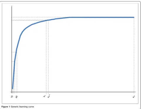
A learning curve is a collection of data points (xj, yj) that in this case describe how the performance of a clas-sifier (yj) is related to training sample sizes (xj), where j = 1 to m, m being the total number of instances. These learning curves can typically be divided into three sec-tions: In the first section, the classification performance increases rapidly with an increase in the size of the training set; the second section is characterized by a turning point where the increase in performance is less rapid and a final section where the classifier has reached its efficiency threshold, i.e. no (or only marginal) improvement in performance is observed with increas-ing trainincreas-ing set size. Figure 1 is an example of a learnincreas-ing curve.
Mukherjee et al. experimented with fitting inverse power laws to empirical learning curves to forecast the performance at larger sample sizes [1]. They have also discussed a permutation test procedure to assess the sta-tistical significance of classification performance for a given dataset size. The method was tested on several relatively small microarray data sets (n = 53 to 280). The differences between the predicted and actual classi-fication errors were found to be in the range of 1%-7%.
Boonyanuntaet al. on the other hand conducted the
curve fitting on several much larger datasets (n = 1,000) using a nonlinear model consistent with the inverse power law [28]. The mean absolute errors were very small, generally below 1%. Our proposed method is similar to that discussed in Mukherjeeet al.with a cou-ple of differences: 1) we conducted weighted curve fit-ting to favor future predictions; 2) we calculated the confidence interval for the fitted curve rather than fit-ting two additional curves for the lower and upper quar-tile data points.
Progressive sampling
amount of computation for a given performance target. For instance, Provostet al. proposed progressive sam-pling using a geometric progression-based samsam-pling schedule [31]. They also explored convergence detection methods for progressive sampling and selected a conver-gence method that used linear regression with local sampling (LRLS). In LRLS, the slope of a linear regres-sion line that has been built with r points sampled around the neighborhood of the last sample size is com-pared to zero. If it is close enough to zero, convergence is detected. The main difference between progressive sampling and SSD of classifiers is that progressive sam-pling assumes there are an unlimited number of anno-tated samples and does not predict the sample size required to reach a specific performance target.
Methods
In this section we describe a new fitting algorithm to predict classifier performance based on a learning curve. This algorithm fits an inverse power law model to a small set of initial points of a learning curve with the
purpose of predicting a classifier’s performance at larger sample sizes. Evaluation was carried out on 12 learning curves at dozens of sample sizes for model fitting and predictions were validated using standard goodness of fit measures.
Algorithm description
The algorithm to model and predict a classifier’s perfor-mance contains three steps:
1) Learning curve creation; 2) Model fitting;
3) Sample size prediction; Learning curve creation
Assuming the target performance measure is classifica-tion, a learning curve that characterizes classification accuracy (Yacc), as a function of the training set size (X) is created. To obtain the data points (xj, yj), classifiers are created and tested at increasing training set sizes xj.
With a batch size k, x j = k·j, j = 1, 2,...,m, i.e.
xj={k, 2k, 3k, ...,k·m}. Classification accuracy points
(yj), i.e. the proportion of correctly classified samples, can be calculated at each training sample sizexjusing an
independent test set or through n-fold cross validation. Model fitting and parameter identification
Learning curves can generally be represented using inverse power law functions [1,27,37,38]. Equation (1) describes the classifier’s accuracy (Yacc) as function of the training sample size × with the parameters a, b, and c representing the minimum achievable error, learning rate and decay rate respectively. The values of the para-meters are expected to differ depending on the dataset, sampling method and the classification algorithm. How-ever, values for parametercare expected to be negative within the range [-1,0]; values foraare expected to be much smaller than 1. The values of Yacc fall between 0
and 1. Yacc grows asymptotically to the maximum
achievable performance, in this case (1-a).
Yacc(x)=f(X;a,b,c)=(1−a)−b·xc (1)
Let us define the setΩas the collection of data points on an empirical learning correspondingto(X,YaccX). Ω
can be partitioned into two sub-sets: Ωt to fit the
model, and Ωtto validate the fitted model. Please note
that in real life applications only Ωt will be available.
For example, at sample size xsΩt= {(xj,yj)|xj≤xs} and
Ωv= {(xj,yj)|xj>xs}.
UsingΩt, we applied nonlinear weighted least squares
optimization together with the nl2sol routine from Port Library[39] to fit the mathematical model from Eq(1) and find the parameter vector β = {a, b, c}.
We also assigned weights to the data points inΩt. As
described earlier, data points on the learning curve associates with sample sizes; we postulated that the clas-sifier performance at a larger training sample size is more indicative of the classifier’s future performance. To account for this, a data point (xj, yj)ÎΩtis assigned the
normalized weightj/mwheremis the cardinality ofΩ. Performance prediction
In this step, the mathematical model (Eq.(1)) together with the estimated parameters {a, b, c} are applied to unseen sample sizes and the resulting prediction is compared with the data points inΩv. In other words, the fitted curve is
used to extrapolate the classifier’s performance at larger sample sizes. Additionally, the 95% confidence interval of the estimated accuracyyˆs is also calculated by using
Hes-sian matrix and the second-order derivatives on the func-tion describing the curve. See appendix1 (addifunc-tional file 1) for more details on the implementation of the methods.
Evaluation
Datasets
We evaluated our algorithm using three sets of data. In the first two sets (D1 and D2), observations are
smoking-related sentences from a set of patient
dis-charge summaries from the Partners Health Care’s
research patient data repository (RPDR). Each observa-tion was manually annotated with smoking status. D1 contains 7,016 sentences and 350 word features to
dis-tinguish between smokers (5,333 sentences) and non
smokers (1,683 sentences). D2 contains 8,449 sentences, 350 word features to discriminate betweenpast smokers (5,109 sentences) and current smokers (3,340 sentences).
The third data set (D3) is thewaveform-5000 dataset from the UCI machine learning repository [40] which contains 5,000 instances, 21 features and three classes of waves (1657 instances of w1, 1647 of w2, and 1696 of w3). The classification goal is to perform binary classifi-cation to discriminate the first class of waves from the other two.
Each dataset was randomly split into a training set and a testing set. Test sets for D1 and D2 contained 1,000 instances each while 2,500 instances were set apart as test set in D3. On the three datasets, we used 4 different sampling methods - three active learning algorithms and a random selection (passive) - together with a support vector machine classifier with linear kernel from WEKA [41] (complexity constant was set to 1, epsilon set to 1,0 E-12, tolerance parameter 1,0E-3, and normalization/ standardization options were turned off) to generate a total of 12 actual learning curves for Yacc. The active learning methods used are:
• Distance (DIST), a simple margin method which
samples training instances based on their proximity to a support vector machine (SVM) hyperplane;
• Diversity (DIV) which selects instances based on their diversity/dissimilarity from instances in the train-ing set. Diversity is measured as the simple cosine dis-tance between the candidate insdis-tances and the already selected set of instances in order to reduce information redundancy; and
•Combined method (CMB) which is a combination of both DIST and DIV methods.
The initial sample size is set to 16 with an increment size of 16 as well, i.e. k = 16. Detailed information about the three algorithms can be found in appendix 2 (see additional file 2) and in literature [10,35,42].
Each experiment was repeated 100 times and Yacc
averaged at each batch size over the 100 runs to obtain data points(xj, yj) of the learning curve.
Goodness of fit measures
Two goodness of fit measurements, mean absolute error (MAE) (Eq.(2)) and root mean squared error (RMSE) (Eq.(3)), were used to evaluate the fitted function onΩv.
MAE is the average absolute value of the difference between the observed accuracy (yj) and the predicted
values of the difference between the observed accuracy (yj) and the predicted accuracy (
yj). RMSE and MAE
values of close to zero indicate a better fit. Using ||Ωv||
to represent the cardinality ofΩv, MAE and RMSE are computed as follows:
MAE= 1
|v| m
(xj,yj)∈v |yj−
∧
yj|,∀ xj,yj
∈ v (2)
RMSE= m (xj,yj)∈v
yj−∧yj
2
|v |
,∀ xj,yj
∈ v
(3)
On each curve, we started the curve fitting and pre-diction experiment at |Ωt| = 5, i.e. at the sample size of
80 instances. In the subsequent experiments, the |Ωt|
was increased by 1 until it reached 62 points, i.e. at the sample size of 992 instances.
To evaluate our method, we used as baseline the non-weighted least squares optimization algorithm described by Mukherjeeet al[1]. Paired t-test was used to com-pare the RMSE and MAE between both methods for all experiments. The alternative hypothesis is that the means of the RMSE and MAE of the baseline method is greater than those of our weighted fitting method.
Results
Using the 3 datasets and 4 sampling methods, 12 actual learning curves are generated. We fitted the inverse power law model to each of the curves, using an increasing number of data points (m = 80-992 in D1 and D2, m = 80-480 in D3). A total of 568 experiments were conducted. In each experiment, the predicted per-formance was compared to the actual observed performance.
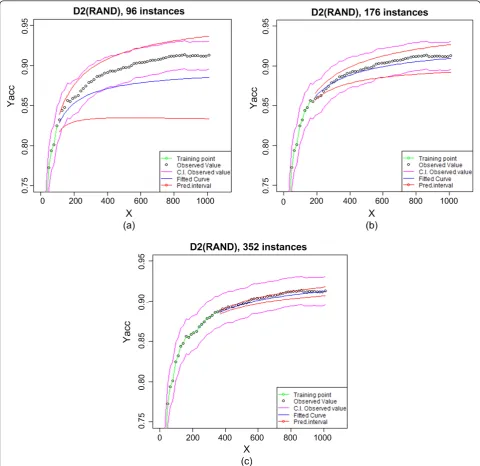
Figure 2 shows the curve fitting and prediction results for the random sampling learning curve using D2 data at different sample sizes. In Figure 2a the curve was fitted using 6 data points; the predicted curve (blue) deviates slightly from the actual data points (black), though the actual data points do fall in the relatively large confidence interval (red). As expected, the devia-tion and confidence interval are both larger as we pro-ject further into the larger sample sizes. In 2b, with 11 data points for fitting, the predicted curve closely resem-bles the observed data and the confidence interval is much narrower. In 2c with 22 data points, the predicted curve is even closer to the actual observations with a very narrow confidence interval.
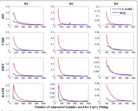
Figure 3 illustrates the width of the confidence interval and MAE at various sample sizes. When the model is fitted with a small number of annotated samples, we
can observe that the confidence interval width and MAE in most of the cases have larger values. As the sample size increases and the prediction accuracy improves, both confidence interval width and MAE values become smaller within a couple of exceptions. At large sample sizes, confidence intervals are very narrow and residual values very small. Both Figures 2 and 3 suggest that the confidence interval width relates to MAE and prediction accuracy.
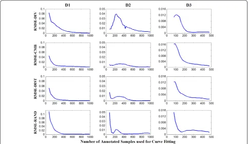
Similarly, Figure 4 shows RMSE for the predicted values on the 12 learning curves with gradually increas-ing sample sizes used for curve fittincreas-ing. Regardincreas-ing fittincreas-ing samples sizes, we can observe a rapid decrease in RMSE and MAE from 80 to 200 instances. From 200 to the end of the curves, values stay relatively constant and close to zero with a few exceptions. The smallest MAE and RMSE were obtained from the D3 dataset on all the learning curves, followed by the learning curves on the D2 dataset. For all datasets RMSE and MAE have simi-lar values with RMSE sometimes being slightly simi-larger.
On Figure 2 and 5, it can be observed that the width of the observed confidence intervals changes only slightly along the learning curves, showing that perfor-mance variance among experiments are not strongly impacted by the sample size. On the other hand, the predicted confidence interval narrows dramatically as more samples are used and the prediction becomes more accurate.
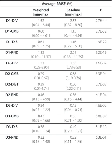
We also compared our algorithm with the un-weighted algorithm. Table 1 shows average values of RMSE for the baseline un-weighted and our weighted method; min and max values are also provided. In all cases, our weighted fitting method had lower RMSE than baseline method with the exception of one tie. We pooled the RMSE values and conducted a paired t-test. The difference between the weighted fitting method and the baseline method is statistically significant (p < 0.05). We conducted a similar analysis comparing the MAE between the two methods and obtained similar results.
Discussion
In this paper we described a relatively simple method to predict a classifier’s performance for a given sample size, through the creation and modelling of a learning curve. As prior research suggests, the learning curves of machine classifiers generally follow the inverse-power law [1,27]. Given the purpose of predicting future per-formance, our method assigned higher weights to data points associated with larger sample size. In evaluation, the weighted methods resulted in more accurate predic-tion (p < 0.05) than the un-weighted method described by Mukherjee et al.
learning algorithms. Prior studies typically used a single type of data (e.g. microarray or text) and a single type of sampling algorithm (i.e. random sampling). By using a variety of data and sampling methods, we were able to test our method on a diverse collection of learning curves and assess its generalizability. For the majority of curves, the RMSE fell below 0.01, within a relative small sample size of 200 used for curve fitting. We observed minimal differences between values of RMSE and MAE which indicates a low variance of the errors.
Our method also provides the confidence intervals of the predicted curves. As shown in Figure 2, the width of
the confidence interval negatively correlates with the prediction accuracy. When the predicted value deviates more from the actual observation, the confidence inter-val tends to be wider. As such, the confidence interinter-val provides an additional measure to help users make the decision in selecting a sample size for additional annota-tion and classificaannota-tion. In our study, confidence intervals were calculated using a variance-covariance matrix on the fitted parameters. Prior studies have stated that the variance is not an unbiased estimator when a model is tested on new data [1]. Hence, our confidence intervals may sometimes be optimistic.
A major limitation of the methods is that an initial set of annotated data is needed. This is a shortcoming shared by other SSD methods for machine classifiers. On the other hand, depending on what confidence interval is deemed acceptable, the initial annotated sam-ple can be of moderate size (e.g.n= 100~200).
The initial set of annotated data is used to create a learning curve. The curve contains
jdata points with a starting sample size of m0 and a
step size ofk. The total sample sizem = m0 + (j-1)*k.
The values ofm0 andkare determined by users. When
m0andkare assigned the same value,m = j*k. In active
learning, a typical experiment may assign m0 as 16 or
32 andkas 16 or 32. For very small data sets, one may consider usem0 = 4 and k= 4. Empirically, we found
that j needed to be greater than or equal to 5 for the curve fitting to be effective.
In many studies, as well as ours, the learning curves appear to be smooth because each data point on the
curve is assigned the average value from multiple experiments (e.g. 10-fold cross validation repeated 100 times). With fewer experiments (e.g. 1 round of training and testing per data point), the curve will not be as smooth. We expect the model fitting to be more accu-rate and the confidence interval to be narrower on smoother curves, though the fitting process remains the same for the less smooth curves.
Although the curve fitting can be done in real time, the time to create the learning curve depends on the classification task, batch size, feature number, processing time of the machine among others. The longest experi-ment we performed to create a learning curve using active learning as sample selection method run on a sin-gle core laptop for several days, though most experi-ments needed only a few hours.
For future work, we intend to integrate the function to predict sample size into our NLP software. The purpose is to guide users in text mining and annotation tasks. In
Figure 4RMSE for predicted values on the three datasets.
clinical NLP research, annotation is usually expensive and the sample size decision is often made based on budget rather than expected performance. It is common for researchers to select an initial number of samples in an ad hoc fashion to annotate data and train a model. They then increase the number of annotations if the tar-get performance could not be reached, based on the vague but generally correct belief that performance will improve with a larger sample size. The amount of improvement though cannot be known without the modelling effort we describe in this paper. Predicting the classification performance for a particular sample size would allow users to evaluate the cost effectiveness of additional annotations in study design. Specifically, we plan for it to be incorporated as part of an active learning and/or interactive learning process.
Conclusions
This paper describes a simple sample size prediction algorithm that conducts weighted fitting of learning curves. When tested on free text and waveform classifi-cation with active and passive sampling methods, the algorithm outperformed the un-weighted algorithm described in previous literature in terms of goodness of
fit measures. This algorithm can help users make an informed decision in sample size selection for machine learning tasks, especially when annotated data are expensive to obtain.
Additional material
Additional file 1: Appendix1 is a PDF file with the main lines of R code that implements curve fitting using inverse power models.
Additional file 2: Appendix 2 is a PDF file that contains more details about the active learning methods used to generate the learning curves.
Acknowledgements
The authors wish to acknowledge CONICYT (Chilean National Council for Science and Technology Research), MECESUP program, and Universidad de Concepcion for their support to this research. This research was funded in part by CHIR HIR 08-374 and VINCI HIR-08-204.
Author details
1Dep. Ing. Eléctrica, Facultad de Ingeniería, Universidad de Concepción, Concepción, Chile.2Department of Biomedical Informatics, University of Utah, Salt Lake City, Utah, USA.3Department of Medicine, Beth Israel Deaconess Medical Center and Harvard Medical School, Boston, MA, USA.
Authors’contributions
QZ and RLF conceived the study. SK and RLF designed and implemented experiments. SK and RLF analyzed data and performed statistical analysis. QZ and LN participated in study design and supervised experiments and data analysis. RLF drafted the manuscript. Both SK and QZ had full access to all of the data and made critical revisions to the manuscript. All authors read and approved the final manuscript.
Competing interests
The authors declare that they have no competing interests.
Received: 30 June 2011 Accepted: 15 February 2012 Published: 15 February 2012
References
1. Mukherjee S, Tamayo P, Rogers S, Rifkin R, Engle A, Campbell C, Golub TR, Mesirov JP:Estimating dataset size requirements for classifying DNA microarray data.J Comput Biol2003,10(2):119-142.
2. Dobbin K, Zhao Y, Simon R:How Large a Training Set is Needed to Develop a Classifier for Microarray Data?Clinical Cancer Research2008,
14(1):108-114.
3. Tam VH, Kabbara S, Yeh RF, Leary RH:Impact of sample size on the performance of multiple-model pharmacokinetic simulations.
Antimicrobial agents and chemotherapy2006,50(11):3950-3952.
4. Kim S-Y:Effects of sample size on robustness and prediction accuracy of a prognostic gene signature.BMC bioinformatics2009,10(1):147. 5. Kalayeh HM, Landgrebe DA:Predicting the Required Number of Training
Samples.Pattern Analysis and Machine Intelligence, IEEE Transactions on 1983,5(6):664-667.
6. Nigam K, McCallum AK, Thrun S, Mitchell T:Text Classification from Labeled and Unlabeled Documents using EM.Mach Learn2000, 39(2-3):103-134.
7. Vlachos A:A stopping criterion for active learning.Computer Speech and Language2008,22(3):295-312.
8. Olsson F, Tomanek K:An intrinsic stopping criterion for committee-based active learning.Proceedings of the Thirteenth Conference on Computational Natural Language LearningBoulder, Colorado: Association for
Computational Linguistics; 2009, 138-146.
9. Zhu J, Wang H, Hovy E, Ma M:Confidence-based stopping criteria for active learning for data annotation.ACM Transactions on Speech and Language Processing (TSLP)2010,6(3):1-24.
Table 1 Average RMSE (%) for baseline and weighted fitting method.
Average RMSE (%)
Weighted [min-max] Baseline [min-max] P D1-DIV 1.52
[0.04 - 8.44]
2.57 [0.82 - 8.70]
2.7E-44
D1-CMB 0.60
[0.06 - 4.61]
1.15 [0.44 - 4.94]
2.7E-32
D1-DIS 0.61
[0.09 - 5.25]
1.16 [0.22 - 5.50]
1.9E-22
D1-RND 1.15
[0.10 - 11.37]
2.01 [0.38 - 11.29]
8.2E-19 D2-DIV 1.33 [0.28-3.95] 1.63 [0.73-3.53] 4.6E-09 D2-CMB 0.29 [0.01-0.67] 0.38 [0.19-0.76] 3.3E-04 D2-DIST 0.39 [0.04-1.74] 0.50 [0.22-2.11] 2.7E-03 D2-RND 0.46
[0.13 - 4.99]
0.56 [0.16 - 4.44]
6.1E-04
D3-DIV 0.34
[0.05 - 1.22]
0.43 [0.04 - 0.93]
4.6E-02
D3-CMB 0.47
[0.09 - 1.66]
0.65 [0.21 - 1.60]
6.0E-09
D3-DIS 0.38
[0.10 - 1.24]
0.49 [0.20 - 1.21]
5.1E-10
D3-RND 0.32
[0.15 - 1.48]
0.32 [0.11 - 1.75]
6.3E-01
10. Figueroa RL, Zeng-Treitler Q:Exploring Active Learning in Medical Text Classification.Poster session presented at: AMIA 2009 Annual Symposium in Biomedical and Health InformaticsSan Francisco, CA, USA; 2009. 11. Kandula S, Figueroa R, Zeng-Treitler Q:Predicting Outcome Measures in
Active Learning.Poster Session presented at: MEDINFO 2010 13th World Congress on MEdical InformaticsCape Town, South Africa; 2010.
12. Maxwell SE, Kelley K, Rausch JR:Sample size planning for statistical power and accuracy in parameter estimation.Annual review of psychology2008,
59:537-563.
13. Adcock CJ:Sample size determination: a review.Journal of the Royal Statistical Society: Series D (The Statistician)1997,46(2):261-283. 14. Lenth RV:Some Practical Guidelines for Effective Sample Size
Determination.The American Statistician2001,55(3):187-193.
15. Briggs AH, Gray AM:Power and Sample Size Calculations for Stochastic Cost-Effectiveness Analysis.Medical Decision Making1998,18(2):S81-S92. 16. Carneiro AV:Estimating sample size in clinical studies: basic
methodological principles.Rev Port Cardiol2003,22(12):1513-1521. 17. Cohen J:Statistical Power Analysis for the Behavioural Sciences.Hillsdale,
NJ: Lawrence Erlbaum Associates; 1988.
18. Scheinin I, Ferreira JA, Knuutila S, Meijer GA, van de Wiel MA, Ylstra B:
CGHpower: exploring sample size calculations for chromosomal copy number experiments.BMC bioinformatics2010,11:331.
19. Eng J:Sample size estimation: how many individuals should be studied?
Radiology2003,227(2):309-313.
20. Walters SJ:Sample size and power estimation for studies with health related quality of life outcomes: a comparison of four methods using the SF-36.Health and quality of life outcomes2004,2:26.
21. Cai J, Zeng D:Sample size/power calculation for case-cohort studies.
Biometrics2004,60(4):1015-1024.
22. Algina J, Moulder BC, Moser BK:Sample Size Requirements for Accurate Estimation of Squared Semi-Partial Correlation Coefficients.Multivariate Behavioral Research2002,37(1):37-57.
23. Stalbovskaya V, Hamadicharef B, Ifeachor E:Sample Size Determination using ROC Analysis.3rd International Conference on Computational Intelligence in Medicine and Healthcare (CIMED2007): 20072007. 24. Beal SL:Sample Size Determination for Confidence Intervals on the
Population Mean and on the Difference Between Two Population Means.Biometrics1989,45(3):969-977.
25. Jiroutek MR, Muller KE, Kupper LL, Stewart PW:A New Method for Choosing Sample Size for Confidence Interval-Based Inferences.
Biometrics2003,59(3):580-590.
26. Fukunaga K, Hayes R:Effects of sample size in classifier design.Pattern Analysis and Machine Intelligence, IEEE Transactions on1989,11(8):873-885. 27. Cortes C, Jackel LD, Solla SA, Vapnik V, Denker JS:Learning Curves:
Asymptotic Values and Rate of Convergence.San Francisco, CA. USA.: Morgan Kaufmann Publishers; 1994VI.
28. Boonyanunta N, Zeephongsekul P:Predicting the Relationship Between the Size of Training Sample and the Predictive Power of Classifiers.In Knowledge-Based Intelligent Information and Engineering Systems. Volume 3215.Springer Berlin/Heidelberg; 2004:529-535.
29. Hess KR, Wei C:Learning Curves in Classification With Microarray Data.
Seminars in oncology2010,37(1):65-68.
30. Last M:Predicting and Optimizing Classifier Utility with the Power Law.
Proceedings of the Seventh IEEE International Conference on Data Mining WorkshopsIEEE Computer Society; 2007, 219-224.
31. Provost F, Jensen D, Oates T:Efficient progressive sampling.Proceedings of the fifth ACM SIGKDD international conference on Knowledge discovery and data miningSan Diego, California, United States: ACM; 1999.
32. Warmuth MK, Liao J, Ratsch G, Mathieson M, Putta S, Lemmen C:Active learning with support vector machines in the drug discovery process.J Chem Inf Comput Sci2003,43(2):667-673.
33. Liu Y:Active learning with support vector machine applied to gene expression data for cancer classification.J Chem Inf Comput Sci2004,
44(6):1936-1941.
34. Li M, Sethi IK:Confidence-based active learning.Pattern Analysis and Machine Intelligence, IEEE Transactions on2006,28(8):1251-1261.
35. Brinker K:Incorporating Diversity in Active Learning with Support Vector Machines.Proceedings of the Twentieth International Conference on Machine Learning (ICML): 20032003, 59-66.
36. Yuan J, Zhou X, Zhang J, Wang M, Zhang Q, Wang W, Shi B:Positive Sample Enhanced Angle-Diversity Active Learning for SVM Based Image
Retrieval.Proceedings of the IEEE International Conference on Multimedia and Expo (ICME 2007): 20072007, 2202-2205.
37. Yelle LE:The Learning Curve: Historical Review and Comprehensive Survey.Decision Sciences1979,10(2):302-327.
38. Ramsay C, Grant A, Wallace S, Garthwaite P, Monk A, Russell I:Statistical assessment of the learning curves of health technologies.Health Technology Assessment2001,5(12).
39. Dennis JE, Gay DM, Welsch RE:Algorithm 573: NL2SOL - An Adaptive Nonlinear Least-Squares Algorithm [E4].ACM Transactions on Mathematical Software1981,7(3):369-383.
40. UCI Machine Learning Repository.[http://www.ics.uci.edu/~mlearn/ MLRepository.html].
41. Weka—Machine Learning Software in Java.[http://weka.wiki.sourceforge. net/].
42. Tong S, Koller D:Support Vector Machine Active Learning with Applications to Text Classification.Journal of Machine Learning Research 2001,2:45-66.
Pre-publication history
The pre-publication history for this paper can be accessed here: http://www.biomedcentral.com/1472-6947/12/8/prepub
doi:10.1186/1472-6947-12-8
Cite this article as:Figueroaet al.:Predicting sample size required for
classification performance.BMC Medical Informatics and Decision Making 201212:8.
Submit your next manuscript to BioMed Central and take full advantage of:
• Convenient online submission
• Thorough peer review
• No space constraints or color figure charges
• Immediate publication on acceptance
• Inclusion in PubMed, CAS, Scopus and Google Scholar
• Research which is freely available for redistribution