Proceedings of NAACL-HLT 2018, pages 106–113
Accelerating NMT Batched Beam Decoding
with LMBR Posteriors for Deployment
Gonzalo Iglesias† William Tambellini† Adri`a De Gispert†‡ Eva Hasler† Bill Byrne†‡
†SDL Research
{giglesias|wtambellini|agispert|ehasler|bbyrne}@sdl.com
‡Department of Engineering, University of Cambridge, U.K.
Abstract
We describe a batched beam decoding algo-rithm for NMT with LMBR n-gram posteri-ors, showing that LMBR techniques still yield gains on top of the best recently reported re-sults with Transformers. We also discuss ac-celeration strategies for deployment, and the effect of the beam size and batching on mem-ory and speed.
1 Introduction
The advent of Neural Machine Translation (NMT) has revolutionized the market. Objective improve-ments (Sutskever et al., 2014; Bahdanau et al.,
2015;Sennrich et al.,2016b;Gehring et al.,2017;
Vaswani et al., 2017) and a fair amount of neu-ral hype have increased the pressure on companies offering Machine Translation services to shift as quickly as possible to this new paradigm.
Such a radical change entails non-trivial chal-lenges for deployment; consumers certainly look forward to better translation quality, but do not want to lose all the good features that have been developed over the years along with SMT tech-nology. With NMT, real time decoding is chal-lenging without GPUs, and still an avenue for re-search (Devlin, 2017). Great speeds have been reported by Junczys-Dowmunt et al. (2016) on GPUs, for which batching queries to the neural model is essential. Disk usage and memory foot-print of pure neural systems are certainly lower than that of SMT systems, but at the same time GPU memory is limited and high-end GPUs are expensive.
Further to that, consumers still need the abil-ity to constrain translations; in particular, brand-related information is often as important for com-panies as translation quality itself, and is cur-rently under investigation (Chatterjee et al.,2017;
Hokamp and Liu, 2017; Hasler et al., 2018). It is also well known that pure neural systems
reach very high fluency, often sacrificing ade-quacy (Tu et al.,2017;Zhang et al.,2017;Koehn and Knowles, 2017), and have been reported to behave badly under noisy conditions (Belinkov and Bisk,2018). Stahlberg et al. (2017) show an effective way to counter these problems by tak-ing advantage of the higher adequacy inherent to SMT systems via Lattice Minimum Bayes Risk (LMBR) decoding (Tromble et al., 2008). This makes the system more robust to pitfalls, such as over- and under-generation (Feng et al.,2016;
Meng et al.,2016;Tu et al.,2016) which is impor-tant for commercial applications.
In this paper, we describe a batched beam de-coding algorithm that uses NMT models with LMBR n-gram posterior probabilities (Stahlberg et al., 2017). Batching in NMT beam decod-ing has been mentioned or assumed in the litera-ture, e.g. (Devlin,2017;Junczys-Dowmunt et al.,
2016), but to the best of our knowledge it has not been formally described, and there are interesting aspects for deployment worth taking into consid-eration.
We also report on the effect of LMBR poste-riors on state-of-the-art neural systems, for five translation tasks. Finally, we discuss how to pre-pare (LMBR-based) NMT systems for deploy-ment, and how our batching algorithm performs in terms of memory and speed.
2 Neural Machine Translation and LMBR
Given a source sentence x, a sequence-to-sequence NMT model scores a candidate transla-tion sentencey=yT
1 withT words as:
PN M T(yT1|x) = T
Y
t=1
PN M T(yt|y1t−1,x) (1)
where PN M T(yt|y1t−1,x) uses a neural func-tion fN M T(·). To account for batching B
ral queries together, our abstract function takes the form offN M T(St−1,yt−1,A) whereSt−1 is the previous batch state withB state vectors in rows,
yt−1 is a vector with the B preceding generated target words, andA is a matrix with the annota-tions (Bahdanau et al.,2015) of a source sentence. The model has a vocabulary sizeV.
The implementation of this function is deter-mined by the architecture of specific models. The most successful ones in the literature typically share in common an attention mechanism that de-termines which source word to focus on, informed byAandSt−1. Bahdanau et al.(2015) use recur-rent layers to both computeAand the next target word yt. Gehring et al.(2017) use convolutional layers instead, andVaswani et al.(2017) prescind from GRU or LSTM layers, relying heavily on multi-layered attention mechanisms, stateful only on the translation side. Finally, this function can also represent an ensemble of neural models.
Lattice Minimum Bayes Risk decoding com-putes n-gram posterior probabilities from an evi-dence spaceand uses them to score a hypothesis space (Kumar and Byrne, 2004; Tromble et al.,
2008;Blackwood et al.,2010). It improves single SMT systems, and also lends itself quite nicely to system combination (Sim et al.,2007;de Gispert et al.,2009). Stahlberg et al.(2017) have recently shown a way to use it with NMT decoding: a tra-ditional SMT system is first used to create an evi-dence spaceϕe, and the NMT space is then scored left-to-right with both the NMT model(s) and the n-gram posteriors gathered from ϕe. More for-mally:
ˆ
y= arg max y
T
X
t=1 (
L(ytt−−n1,yt)
z }| {
Θ0+ 4
X
n=1
ΘnPLM BR(ytt−n|ϕe)
+λlogPN M T(yt|y1t−1,x)) (2)
For our purposesLis arranged as a matrix with each row uniquely associated to an n-gram history identified inϕe: each row contains scores for any wordyin the NMT vocabulary.
L can be precomputed very efficiently, and stored in the GPU memory. The number of distinct n-gram histories is typically no more than500for our phrase-based decoder producing200 hypothe-ses. Notice that such a matrix only containing
PLM BR contributions would be very sparse, but
it turns into a dense matrix with the summation ofΘ0. Both sparse and dense operations can be performed on the GPU. We have found it more ef-ficient to compute first all the sparse operations on CPU, and then upload to the GPU memory and sum the constantΘ0in GPU1.
3 NMT batched beam decoding
Algorithm 1 describes NMT decoding with LMBR posteriors using beam sizeB equal to the
batch size. Lines 2-5 initialize the decoder; the number of time stepsT is usually a heuristic
func-tion of the source length. qwill keep track of the
Bbest scores per time step,bandyare indices. Lines 7-16 are the core of the batch decoding procedure. At each time stept, givenSt−1,yt−1 andA,fN M T returns two matrices: Pt, with size
B×V, contains log-probabilities for all possible
candidates in the vocabulary givenBlive
hypothe-ses. Stis the next batch state. Each row in Stis the vector state that corresponds to any candidate in the same row ofPt(line 8).
Lines 9, 10 add the n-gram posterior scores. Given the indices inbandyit is straightforward to read the unique histories for the B open
hy-potheses: the topology of the hypothesis space is that of a tree because an NMT state represents the entire live hypothesis from time step0. Note that btj < B is the index to access the previ-ous word in yt−1. In effect, indices in b func-tion as backpointers, allowing to reconstruct not only n-grams per time step, but also complete hypotheses. As discussed for Equation 2, these histories are associated to rows in our matrix L. Function GETMATRIXBYROWS(·)simply creates a new matrix of sizeB ×V by fetching thoseB
rows fromL. This new matrix is summed to Pt (line10).
In line 11, we get the indices and scores in Pt+q0t−1 of the top B hypotheses. These best hypotheses could come from any row inPt. For example, all B best hypotheses could have been found in row 0. In that case, the new batch state to be used in the next time step should contain copies of row 0 in the otherB−1rows. This is achieved again with GETMATRIXBYROWS(·)in line 12.
Finally, lines 13-16 identify whether there are any end-of-sentence (EOS) candidates; the
corre-1Ideally we would want to keepLas a sparse matrix and
Algorithm 1Batch decoding with LMBR n-gram posteriors 1: procedureDECODENMT(x,L)
2: T ←Maximum target hypothesis length
3: b,y,qindices and scores, withb0 ←0,y0←0,q0←0
4: A←Annotations for source sentence x 5: S0←Initial decoder state
6: F ={} . Set of EOS survivors
7: fort = 1 to T do
8: Pt,St←fN M T(St−1,yt−1,A)
9: h←Bhistories identified throughb,yandt
10: Pt←Pt+GETMATRIXBYROWS(L,h) .Add LMBR contributions
11: bt,yt,qt← TOPB(Pt+q0t−1)
12: St← GETMATRIXBYROWS(St,bt)
13: forj = 0 to B−1do 14: ifytj=EOSthen
15: F ←F ∪({t, j, qtj}) .Track indices and score
16: qtj ← −∞ .Mask out to prevent hypothesis extension
17: returnGETBESTHYPOTHESIS(F,b,y)
sponding indices and score are pushed into stack
F and these candidates are masked out (i.e. set
to−∞) to prevent further expansion. In line17, GETBESTHYPOTHESIS(F) traces backwards the best hypothesis inF, again using indices inband y. Optionally, normalization by hypothesis length happens in this step.
It is worth noting that:
1. If we drop lines 9, 10 we have a pure left-to-right NMT batched beam decoder.
2. Applying a constraint (e.g. for lattice rescor-ing or other user constraints) involves mask-ing out scores inPtbefore line 11.
3. Because the batch size is tied to the beam size, the memory footprint increases with the beam.
4. Due to the beam being used for both EOS and non EOS candidates, it can be argued that this empoverishes the beam and it could be kept in addition to non EOS candidates (either by using a bigger beam, or keeping separately). Empirically we have found that this does not affect quality with real models.
5. The opposite, i.e. that EOS candidates never survive in the beam for T time steps, can
happen, although very infrequently. Several pragmatic backoff strategies can be applied in this situation: for example, running the de-coder for additional time steps, or tracking
all EOS candidates that did not survive in a separate stack and picking the best hypothe-sis from there. We chose the latter.
3.1 Extension to Sentence batching
In addition to batching allB queries to the neural
model needed to compute the next time step for one sentence, we can dosentence batching: this is, we translateNsentences simultaneously, batching B×N queries per time step.
With small modifications, Algorithm 1 can be easily extended to handle sentence batching. If the number of sentences isN,
1. Instead of one setFto store EOS candidates,
we needF1...FN sets.
2. For every time step, bt,yt and qt need to be matrices instead of vectors, and minor changes are required in TOPB(·)to fetch the best candidates per sentence efficiently.
3. PtandStcan remain as matrices, in which case the new batch size is simplyB·N.
4. The heuristic function used to computeT is typically sentence specific.
4 Experiments
4.1 Experimental Setup
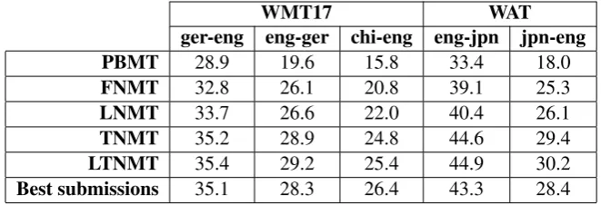
WMT17 WAT ger-eng eng-ger chi-eng eng-jpn jpn-eng PBMT 28.9 19.6 15.8 33.4 18.0
FNMT 32.8 26.1 20.8 39.1 25.3
LNMT 33.7 26.6 22.0 40.4 26.1
TNMT 35.2 28.9 24.8 44.6 29.4
LTNMT 35.4 29.2 25.4 44.9 30.2
[image:4.595.133.464.62.175.2]Best submissions 35.1 28.3 26.4 43.3 28.4
Table 1: Quality assessment of our NMT systems with and without LMBR posteriors for GRU-based (FNMT, LNMT) and Transformer models (TNMT, LTNMT). Cased BLEU scores reported on5translation tasks.The exact
PBMT systems used to compute n-gram posteriors for LNMT and LTNMT systems are also reported. The last row shows scores for the best official submissions to each task.
pairs for the WMT17 task, and Japanese-English and English-Japanese for the WAT task. For the German tasks we use news-test2013 as a de-velopment set, and news-test2017 as a test set; for Chinese-English, we use news-dev2017 as a development set, and news-test2017 as a test set. For Japanese tasks we use the ASPEC cor-pus (Nakazawa et al.,2016).
We use all available data in each task for training. In addition, for German we use back-translation data (Sennrich et al., 2016a). All training data for neural models is preprocessed with the byte pair encoding technique described by Sennrich et al. (2016b). We use Blocks (van Merri¨enboer et al., 2015) with Theano (Bastien et al., 2012) to train attention-based single GRU layer models (Bahdanau et al.,2015), henceforth calledFNMT. The vocabulary size is50K. Trans-former models (Vaswani et al.,2017), called here
TNMT, are trained using the Tensor2Tensor pack-age2with a vocabulary size of30K.
Our proprietary translation system is a mod-ular homegrown tool that supports pure neural decoding (FNMT and TNMT) and with LMBR posteriors (henceforce called LNMT and LT-NMT respectively), and flexibly uses other com-ponents (phrase-based decoding, byte pair encod-ing, etcetera) to seamlessly deploy an end-to-end translation system.
FNMT/LNMT systems use ensembles of 3 neural models unless specified otherwise; TNMT/LTNMT systems decode with 1 to 2 mod-els, each averaging over the last 20 checkpoints.
The Phrase-based decoder (PBMT) uses stan-dard features with one single 5-gram language
2https://github.com/tensorflow/
tensor2tensor
model (Heafield et al., 2013), and is tuned with standard MERT (Och, 2003); n-gram posterior probabilities are computed on-the-fly over rich translation lattices, with size bounded by the PBMT stack and distortion limits. The parameter
λin Equation2is set as 0.5 divided by the number
of models in the ensemble. Empirically we have found this to be a good setting in many tasks.
Unless noted otherwise, the beam size is set to 12 and the NMT beam decoder always batches queries to the neural model. The beam decoder relies on an early preview of ArrayFire 3.6 ( Yala-manchili et al.,2015)3, compiled with CUDA 8.0
libraries. For speed measurements, the decoder uses one single CPU thread. For hardware, we use an Intel Xeon CPU E5-2640 at 2.60GHz. The GPU is a GeForce GTX 1080Ti. We report cased BLEU scores (Papineni et al.,2002), strictly com-parable to the official scores in each task4.
4.2 The effect of LMBR n-gram posteriors
Table1shows contrastive experiments for all five language pair/tasks. We make the following ob-servations:
1. LMBR posteriors show consistent gains on top of the GRU model (LNMT vs FNMT rows), ranging from +0.5BLEU to
+1.2BLEU. This is consistent with the
find-ings reported byStahlberg et al.(2017).
2. The TNMT system boasts improvements across the board, ranging from +1.5BLEU
in German-English to an impressive +4.2BLEU in English-Japanese WAT
3http://arrayfire.org
4http://matrix.statmt.org/ and
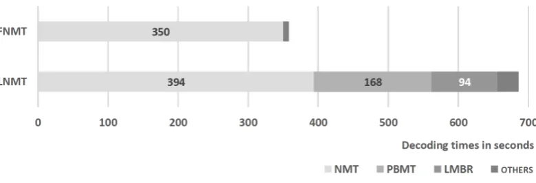
Figure 1: Accelerated FNMT and LNMT decoding times for newstest-2017 test set.
(TNMT vs LNMT). This is in line with findings by Vaswani et al. (2017) and sets new very strong baselines to improve on.
3. Further, applying LMBR posteriors along with the Transformer model yields gains in all tasks (LTNMT vs TNMT), up to +0.8BLEU in Japanese-English.
Interest-ingly, while we find that rescoring PBMT lat-tices (Stahlberg et al.,2016) with GRU mod-els yields similar improvements to those re-ported byStahlberg et al.(2017), we did not find gains when rescoring with the stronger TNMT models instead.
4.3 Accelerating FNMT and LNMT systems for deployment
There is no particular constraint on speed for the research systems reported in Table1. We now ad-dress the question of deploying NMT systems so that MT users get the best quality improvements at real-time speed and with acceptable memory footprint. As an example, we analyse in detail the English-German FNMT and LNMT case and discuss the main trade-offs if one wanted to ac-celerate them. Although the actual measurements vary across all our productised NMT engines, the trends are similar to the ones reported here.
In this particular case we specify a beam width of 0.01 for early pruning (Wu et al., 2016; De-laney et al., 2006) and reduce the beam size to 4. We also shrink the ensemble into one single big model5 using the data-free shrinking method
described by Stahlberg and Byrne(2017), an in-expensive way to improve both speed and GPU memory footprint.
5The file size of each3individual models of the ensemble
is 510MB; the size of the shrunken model is 1.2GB.
In addition, for LNMT systems we tune phrase-based decoder parameters such as the distortion limit, the number of translations per source phrase and the stack limit. To compute n-gram posteri-ors we now only take a200-best from the phrase-based translation lattice.
Table2shows a contrast of our English-German WMT17 research systems versus the respective accelerated ones.
Research Accelerated BLEU speed BLEU speed FNMT 26.1 2207 25.2 9449 LNMT 26.6 263 25.7 4927
Table 2: Cased BLEU scores forresearchvs acceler-atedEnglish-to-German WMT17 systems. Speed re-ported in words per minute.
In the process, both accelerated systems have lost 0.9 BLEU relative to the baseline. As an example, let us break down the effects of accel-erating the LNMT system: using only 200-best hypotheses from the phrase-based translation lat-tice reduces 0.3 BLEU. Replacing the ensemble with a data-free shrunken model reduces another 0.2BLEU and decreasing the beam size reduces 0.4BLEU. The impact of reducing the beam size varies from system to system, although often does not result in substantial quality loss for NMT mod-els (Britz et al.,2017).
[image:5.595.313.520.371.430.2]probabil-Figure 2: Batch beam decoder speed measured over newstest-2017 test set, using the accelerated FNMT system (25.2BLEU for beam size =4).
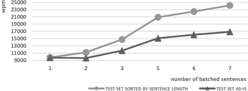
Figure 3: Batch beam decoder speed measured over newstest-2017 test set, using the accelerated eng-ger-wmt17 FNMT system (26.1BLEU) with additional sentence batching, up to7sentences.
ities. In effect, while both are remarkably fast by themselves (e.g. the phrase-based decoder is run-ning at20000wpm), these extra contributions ex-plain most of the speed reduction for the acceler-ated LNMT system. In addition, the beam decoder itself is slightly slower for LNMT than for FNMT. This is mainly due to the computation ofLas ex-plained in Section2. Finally, the respective GPU memory footprints for FNMT and LNMT are4.1 and4.8GB.
4.4 Batched beam decoding and beam size
We next discuss the impact of using batch de-coding and the beam size. To this end we use the accelerated FNMT system (25.2BLEU,9449 wpm) to decode with and without batching; we also widen the beam. Figure2shows the results.
The accelerated system itself with batched beam decoding and beam size of4is3times faster than without batching (3053 wpm). The GPU memory footprint is 1 GB bigger when batching
(4.1vs3.1GB). As can be expected, widening the beam decreases the speed of both decoders. The relative speed-up ratio favours the batch decoder for wider beams, i.e. it is 5 times faster for beam size 12. However, because the batch size is tied to the beam size, this comes at a cost in GPU mem-ory footprint (under8GB).
4.5 Sentence batching
As described in Section3.1, it is straightforward to extend beam batching to sentence batching. Fig-ure3shows the effect of sentence batching up to 7 sentences on our accelerated FNMT system.
[image:6.595.97.497.260.407.2]7 sentences, which approaches the limit of GPU memory.
Note that sentence batching does not change translation quality. For example, when translating 7 sentences, we are effectively batching 28 neural queries per time step. Indeed, each individual sen-tence is still being translated with a beam size of 4.
Figure3also shows the effect of sorting the test set by sentence length. Because sentences have similar lengths, less padding is required and hence we have less wasteful GPU computation. With7 batched sentences the decoder would run at barely 17000wpm, this is,7000wpm less due to not sort-ing by sentence length. A similar strategy is com-mon for neural training (Sutskever et al., 2014;
Morishita et al.,2017).
5 Conclusions
We have described a left-to-right batched beam NMT decoding algorithm that is transparent to the neural model and can be combined with LMBR n-gram posteriors. Our quality assessment with Transformer models (Vaswani et al., 2017) has shown that LMBR posteriors can still improve such a strong baseline in terms of BLEU. Finally, we have also discussed our acceleration strategy for deployment and the effect of batching and the beam size on memory and speed.
References
Dzmitry Bahdanau, Kyunghyun Cho, and Yoshua Ben-gio. 2015. Neural machine translation by jointly learning to align and translate.ICLR.
Fr´ed´eric Bastien, Pascal Lamblin, Razvan Pascanu, James Bergstra, Ian J. Goodfellow, Arnaud Berg-eron, Nicolas Bouchard, and Yoshua Bengio. 2012. Theano: new features and speed improvements. Deep Learning and Unsupervised Feature Learning NIPS 2012 Workshop.
Yonatan Belinkov and Yonatan Bisk. 2018. Synthetic and natural noise both break neural machine transla-tion.ICLR.
Graeme Blackwood, Adri`a Gispert, and William Byrne. 2010. Efficient path counting transducers for minimum bayes-risk decoding of statistical machine translation lattices. In Proceedings of ACL, pages 27–32.
Denny Britz, Anna Goldie, Minh-Thang Luong, and Quoc Le. 2017. Massive exploration of neural ma-chine translation architectures. In Proceedings of EMNLP, pages 1442–1451.
Rajen Chatterjee, Matteo Negri, Marco Turchi, Mar-cello Federico, Lucia Specia, and Fr´ed´eric Blain. 2017. Guiding neural machine translation decoding with external knowledge. InProceedings of WMT, pages 157–168.
Brian Delaney, Wade Shen, and Timothy Anderson. 2006. An efficient graph search decoder for phrase-based statistical machine translation. In Proceed-ings of IWSLT.
Jacob Devlin. 2017. Sharp models on dull hardware: Fast and accurate neural machine translation decod-ing on the cpu. In Proceedings of EMNLP, pages 2820–2825.
Shi Feng, Shujie Liu, Nan Yang, Mu Li, Ming Zhou, and Kenny Q. Zhu. 2016. Improving attention mod-eling with implicit distortion and fertility for ma-chine translation. InProceedings of COLING, pages 3082–3092.
Jonas Gehring, Michael Auli, David Grangier, De-nis Yarats, and Yann N. Dauphin. 2017. Con-volutional sequence to sequence learning. CoRR, abs/1705.03122.
Adri`a de Gispert, Sami Virpioja, Mikko Kurimo, and William Byrne. 2009. Minimum bayes risk com-bination of translation hypotheses from alternative morphological decompositions. InProceedings of NAACL-HLT, pages 73–76.
Eva Hasler, Adri`a de Gispert, Gonzalo Iglesias, and Bill Byrne. 2018. Neural machine translation de-coding with terminology constraints. In Proceed-ings of NAACL-HLT.
Kenneth Heafield, Ivan Pouzyrevsky, Jonathan H. Clark, and Philipp Koehn. 2013. Scalable modified kneser-ney language model estimation. In Proceed-ings of ACL, pages 690–696.
Chris Hokamp and Qun Liu. 2017. Lexically con-strained decoding for sequence generation using grid beam search. InProceedings of ACL, pages 1535– 1546.
Marcin Junczys-Dowmunt, Tomasz Dwojak, and Hieu Hoang. 2016. Is neural machine translation ready for deployment? A case study on 30 translation di-rections.CoRR, abs/1610.01108.
Philipp Koehn and Rebecca Knowles. 2017. Six chal-lenges for neural machine translation. In Pro-ceedings of the First Workshop on Neural Machine Translation, pages 28–39.
Shankar Kumar and William Byrne. 2004. Minimum bayes-risk decoding for statistical machine transla-tion. InProceedings of NAACL-HLT, pages 169– 176.
Bart van Merri¨enboer, Dzmitry Bahdanau, Vincent Dumoulin, Dmitriy Serdyuk, David Warde-Farley, Jan Chorowski, and Yoshua Bengio. 2015. Blocks and fuel: Frameworks for deep learning. CoRR, abs/1506.00619.
Makoto Morishita, Yusuke Oda, Graham Neubig, Koichiro Yoshino, Katsuhito Sudoh, and Satoshi Nakamura. 2017. An empirical study of mini-batch creation strategies for neural machine translation. In Proceedings of the First Workshop on Neural Ma-chine Translation, pages 61–68.
Toshiaki Nakazawa, Manabu Yaguchi, Kiyotaka Uchi-moto, Masao Utiyama, Eiichiro Sumita, Sadao Kurohashi, and Hitoshi Isahara. 2016. ASPEC: Asian scientific paper excerpt corpus. In Proceed-ings of LREC.
Franz Josef Och. 2003. Minimum error rate training in statistical machine translation. InProceedings of ACL, pages 160–167.
Kishore Papineni, Salim Roukos, Todd Ward, and Wei-Jing Zhu. 2002. Bleu: a method for automatic eval-uation of machine translation. In Proceedings of ACL, pages 311–318.
Rico Sennrich, Barry Haddow, and Alexandra Birch. 2016a. Improving neural machine translation mod-els with monolingual data. InProceedings of ACL, pages 86–96.
Rico Sennrich, Barry Haddow, and Alexandra Birch. 2016b. Neural machine translation of rare words with subword units. InProceedings of ACL, pages 1715–1725.
K. C. Sim, W. J. Byrne, M. J. F. Gales, H. Sahbi, and P. C. Woodland. 2007. Consensus network decod-ing for statistical machine translation system combi-nation. InProceedings of ICASSP, volume 4, pages 105–108.
Felix Stahlberg and Bill Byrne. 2017. Unfolding and shrinking neural machine translation ensembles. In Proceedings of EMNLP, pages 1946–1956.
Felix Stahlberg, Adri`a de Gispert, Eva Hasler, and Bill Byrne. 2017. Neural machine translation by minimising the bayes-risk with respect to syntactic translation lattices. In Proceedings of EACL, vol-ume 2, pages 362–368.
Felix Stahlberg, Eva Hasler, Aurelien Waite, and Bill Byrne. 2016. Syntactically guided neural machine translation. InProceedings of ACL, pages 299–305. Ilya Sutskever, Oriol Vinyals, and Quoc V. Le. 2014. Sequence to sequence learning with neural net-works. In Proceedings of NIPS, volume 2, pages 3104–3112, Cambridge, MA, USA. MIT Press. Roy Tromble, Shankar Kumar, Franz Och, and
Wolf-gang Macherey. 2008. Lattice Minimum Bayes-Risk decoding for statistical machine translation. In Proceedings of EMNLP, pages 620–629.
Zhaopeng Tu, Yang Liu, Zhengdong Lu, Xiaohua Liu, and Hang Li. 2017. Context gates for neural ma-chine translation. Transactions of the Association for Computational Linguistics, 5:87–99.
Zhaopeng Tu, Zhengdong Lu, Yang Liu, Xiaohua Liu, and Hang Li. 2016. Modeling coverage for neural machine translation. InProceedings of ACL, pages 76–85.
Ashish Vaswani, Noam Shazeer, Niki Parmar, Jakob Uszkoreit, Llion Jones, Aidan N. Gomez, Lukasz Kaiser, and Illia Polosukhin. 2017. Attention is all you need.CoRR, abs/1706.03762.
Yonghui Wu, Mike Schuster, Zhifeng Chen, Quoc V. Le, Mohammad Norouzi, Wolfgang Macherey, Maxim Krikun, Yuan Cao, Qin Gao, Klaus Macherey, Jeff Klingner, Apurva Shah, Melvin Johnson, Xiaobing Liu, Lukasz Kaiser, Stephan Gouws, Yoshikiyo Kato, Taku Kudo, Hideto Kazawa, Keith Stevens, George Kurian, Nishant Patil, Wei Wang, Cliff Young, Jason Smith, Jason Riesa, Alex Rudnick, Oriol Vinyals, Greg Corrado, Macduff Hughes, and Jeffrey Dean. 2016. Google’s neural machine translation system: Bridging the gap between human and machine translation. CoRR, abs/1609.08144.
Pavan Yalamanchili, Umar Arshad, Zakiuddin Mo-hammed, Pradeep Garigipati, Peter Entschev, Brian Kloppenborg, James Malcolm, and John Melonakos. 2015. ArrayFire - A high performance software library for parallel computing with an easy-to-use API.