JU ETCE 17 21 at SemEval 2019 Task 6: Efficient Machine Learning and Neural Network Approaches for Identifying and Categorizing Offensive Language in Tweets

Proceedings of the 13th International Workshop on Semantic Evaluation (SemEval-2019), pages 662–667 662

JU ETCE 17 21 at SemEval-2019 Task 6: Efficient Machine Learning

and Neural Network Approaches for Identifying and Categorizing

Offensive Language in Tweets

Mainak Pal*_{, Preeti Mukherjee}∗_{, Somnath Banerjee, Sudip Kumar Naskar}

Jadavpur University, Kolkata, India

{mainak.pal08,preetimukherjee08,sb.cse.ju}@gmail.com [email protected]

Abstract

This paper describes our system submissions as part of our participation (team name: JU ETCE 17 21) in the SemEval 2019 shared task 6: “OffensEval: Identifying and Catego-rizing Offensive Language in Social Media”. We participated in all the three sub-tasks: i) Sub-task A: offensive language identification, ii) Sub-task B: automatic categorization of of-fense types, and iii) Sub-task C: ofof-fense target identification. We employed machine learn-ing as well as deep learnlearn-ing approaches for the sub-tasks. We employed Convolutional Neural Network (CNN) and Recursive Neu-ral Network (RNN) Long Short-Term Memory (LSTM) with pre-trained word embeddings. We used both word2vec and Glove pre-trained word embeddings. We obtained the best F1-score using CNN based model for sub-task A, LSTM based model for sub-task B and Lo-gistic Regression based model for sub-task C. Our best submissions achieved 0.7844, 0.5459 and 0.48 F1-scores for sub-task A, sub-task B and sub-task C respectively.

1 Introduction

Today, very large amounts of information are available in online documents. As part of the ef-fort to better organize this information for users, researchers have been actively investigating the problem of automatic text categorization. Tweets are short length pieces of text, usually writ-ten in informal style that contain abbreviations, misspellings and creative syntax (like emoticons, hashtags etc). In this paper we show that our

∗

These two authors have contributed equally

multi-view ensemble approach that leverages sim-ple representations of texts may achieve good re-sults in the task of message polarity classification. We used different machine learning algorithm and neural network approaches for all the tasks which are explained in the subsequent sections. The pa-per is organized as follows: Section 2 lists down the related work and Section 3 describes our ap-proach. Section 4 presents the experiments, results on the development set and discussion about the confusion matrix and Section 5 details about the observation. Section 6 concludes the paper with possible future work.

OffensEval@SemEval-2019 shared task de-scription, data and results are described in the overview paper (Zampieri et al.,2019b).

2 Related Work

Papers published in the last two years include the surveys by (Schmidt and Wiegand, 2017) and (Fortuna and Nunes, 2018), the paper by (Davidson et al., 2017) presenting the Hate Speech Detection dataset used in (Malmasi and Zampieri, 2017) and a few other recent papers such as (ElSherief et al., 2018; Gamb¨ack and Sikdar,2017;Zhang et al.,2018).

A proposal of typology of abusive language sub-tasks is presented in (Waseem et al., 2017). For studies on languages other than English see (Su et al., 2017) on Chinese and (Fiˇser et al.,

high-lighted the challenges of distinguishing between profanity, and threatening language which may not actually contain profane language.

In addition, we would also like to mention the previous editions of related workshops such as TA-COS1_{, Abusive Language Online}2_{, and}

TRAC3and related shared tasks such as GermEval (Wiegand et al., 2018) and TRAC (Kumar et al.,

2018).

3 Methodology and Data

3.1 Data Description

The organizers provided a dataset of 13,240 tweets which were annotated with the following task-specific categories.

• Sub-task A: Offensive language

identifica-tion.

1. Not Offensive (NOT): These posts do not contain offense or profanity.

2. Offensive (OFF): These posts contain offensive language or a targeted (veiled or direct) offense.

• Sub-task B:Automatic categorization of

of-fense types.

1. Targeted Insult and Threats (TIN): A post containing an insult or threat to an individual, a group, or others (see cate-gories in sub-task C).

2. Untargeted (UNT): A post containing non-targeted profanity and swearing.

• Sub-task C:Offense target identification.

1. Individual (IND): The target of the of-fensive post is an individual: a famous person, a named individual or an un-named person interacting in the conver-sation.

2. Group (GRP): The target of the offen-sive post is a group of people consid-ered as a unity due to the same ethnic-ity, gender or sexual orientation, politi-cal affiliation, religious belief, or some-thing else.

1

http://ta-cos.org/ 2

https://sites.google.com/site/ abusivelanguageworkshop2017/

3_{https://sites.google.com/view/trac1/}

home

3. Other (OTH): The target of the offensive post does not belong to any of the pre-vious two categories (e.g., an organiza-tion, a situaorganiza-tion, an event, or an issue).

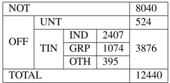
Table 1: Statistics of the training dataset

NOT 8040

OFF

UNT 524

TIN

IND 2407

3876

GRP 1074

OTH 395

TOTAL 12440

The data collection methods used to compile the dataset used in OffensEval is described in

Zampieri et al. (2019a). Table1 provides statis-tics of the training dataset.

3.2 Preprocessing

Raw tweets scraped from twitter generally result in a noisy dataset. This is due to the casual nature of people’s usage of social media. Tweets have certain special characteristics such as re-tweets, emoticons, user mention, etc. which have to be suitably extracted. Therefore, raw twitter data has to be normalized to create a dataset which can be easily learned by various classifiers. We ap-plied an extensive number of pre-processing steps to standardize the dataset and reduce its size. Ini-tially, we performed basic pre-processing opera-tions on tweets which are as follows:

1. Convert the tweets to lower case.

2. Selective removal of special twitter features like URL, User mention, Hash-tags etc. (Cf. Table2)

3. Converting abbreviated negative english words to common negative verbs.

4. Removing special characters and numbers.

5. Tokenization.

Table 2: Regex used for pre-processing

Twitter Feature Regex pattern

URL https?://[ˆ ]+|www.[ˆ ]+

Mention @[A-Za-z0-9]+

3.3 Machine Learning

Most of the machine learning (ML) algorithms are heavily reliant on hand crafted features designed by experts. This makes ML algorithms less gen-eralizable. So we did not use any language spe-cific features. We used various Machine Learning techniques to classify the tweets. When compar-ing various machine learncompar-ing algorithms, baseline provides a point of reference to compare. While developing the models, we employed TextBlob4_as

baseline. We compared the validation result with TextBlob. Textblob is a python library for process-ing textual data. Apart from useful tools such as POS tagging, n-gram,etc. it has a built-in senti-ment classification tool. We also tried a variation for the fine-grained classification task where the predicted output from task A was also added as a feature to the TF-IDF and list specific features. We validated our models using 15% of the train-ing data. We built an ensemble (vottrain-ing) classifier with top 5 models for different types of vectoriz-ers, number of features, n-grams, etc.

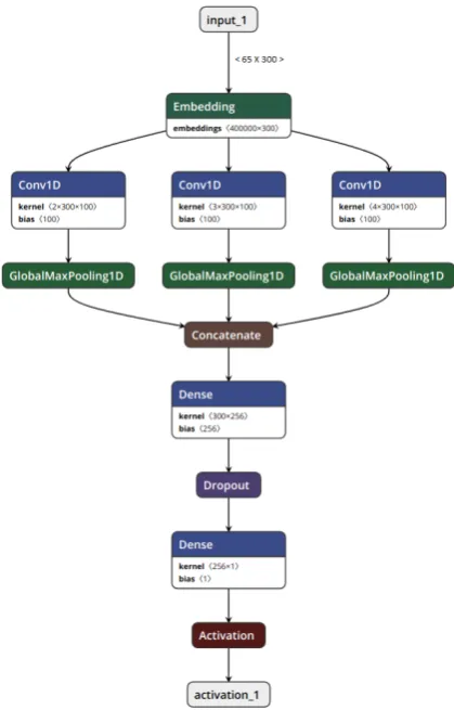
3.4 Convolutional Neural Network

Word embedding: We used Glove5as the vector

representation of the words in tweets. The dimen-sion of the embedding is 300. We fine-tuned the word embedding during the network training.

Network Architecture: As shown in the

Fig-ure 1 embedding layer is used to provide word embedding. We used 300 dimensional word vec-tors for each words. We used 1D CNN on text data represented in word vectors. Filter column width is same as the data column width. It will ensure that matrix will stride vertically only. The padded data of the input text is of size 65x300 for each sentences. Therefore, filter’s column width will be 300. Height is similar to the concept of n-gram. If the filter height is 2, the filter will stride through the document computing the calculations with all the bigrams; if the filter height is 3, it will go through all the trigrams in the document, and so on. The output height is measured by the fol-lowing mathematical expression :

Output height= ((H−hf)/s) + 1

where, H: Input data height hf: Filter height s: Stride size

4

https://textblob.readthedocs.io/en/dev/ 5_{https://nlp.stanford.edu/projects/glove/}

Figure 1: Convolutional Neural Network

Global Max Pooling layer extracts the maxi-mum value from each filter, and the output dimen-sion is 1-dimendimen-sional vector with length as same as the number of filters we applied. This can be directly passed on to a dense layer without flatten-ing.

We implemented the above with bi-gram, tri-gram and four-tri-gram filters. However, this is not linearly stacked layers, but parallel layers. And after convolutional layer and max-pooling layer, it simply concatenated max pooled result from each of bi-gram, tri-gram, and four-gram, then build one output layer on top of them. We added one fully connected hidden layer with dropout just be-fore the output layer. Output layer has just one output node with Sigmoid activation.

3.5 Recurrent Neural Networks

Long Short-Term Memory networks are an exten-sion for RNN. We employed LSTM as RNN ar-chitecture.

Word embedding: Here, we also used Glove

fine-tuned the word embedding during the network training.

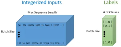
Network Architecture: The matrix contains

400,000 word vectors, each with a dimensionality mentioned above. We imported two different data structures, one was a Python list with the 400,000 words, and another was a400,000×200 dimen-sional embedding matrix that holds all of the word vector values. We defined the necessary hyper-parameters and specified the two placeholders, one for the inputs into the network, and one for the la-bels. The most important part about defining these placeholders was understanding each of their di-mensionality. For both tasks, the output layer con-tained nodes equal to the number of class labels( 2 for task A and B, 3 for task C ).

Figure 2: Vectorized tweets and corresponding la-bels

Each row in the integerized input placeholder represents the integerized representation of each training example that we included in our batch. Hidden state vector can be represented as :

ht=σ(wHht−1+wXxt)

where,wHandwX are weight metrics,xtis a

vec-tor that encapsulates all the information of a spe-cific word.

We also used LSTM network as a module in RNN for better understanding of a sentence. All the vectors are given as a sequence of vectors for a bidirectional LSTM. The representation of a tweet is the representation learned after pass-ing the whole sequence of tokens through the biL-STM. We defined a standard cross entropy loss with a softmax layer put on top of the final pre-diction values. For the optimizer, we used Adam and the default learning rate of 0.001.

4 Results

This section presents the obtained results for the three sub-tasks.

Figure 3: LSTM unit

4.1 Sub-task A:

We implemented all the three systems for this sub-task. For Machine learning, we obtained best results for Count-vectorizer with tri-gram and 90,000 features and with Logistic Regression Classifier. We achieved best results for CNN-Glove with Macro-F1 0.7844 and overall Accu-racy 0.8419. However, due to paucity of time, we were unable to extract the output from our RNN model in the stipulated time frame.

System F1 (macro) Accuracy

All NOT baseline 0.4189 0.7209

All OFF baseline 0.2182 0.2790

ML model 0.7231 0.8105

CNN-glove 0.7844 0.8419

Table 3: Results for Sub-task A.

NOT OFF

Predicted label NOT

OFF

True label

584 36

100 140

Confusion Matrix

0.0 0.2 0.4 0.6 0.8

4.2 Sub-task B:

Our approach was similar to that in the previous Sub-task. We changed the training set and la-bels of the same appropriately, and got our results. We used 2 class layers for training.We observed that the model gives better validation accuracy while fitted with cleaned data parsing with@user. While training the RNN network, we used alterna-tive targeted and non-targeted tweets from anno-tated data. We obtained best results for RNN with Macro-F1 0.54587543782 and overall Accuracy 0.804166666667. The Hyper-parameters of this model are: Batchsize:24, LSTM Units:64, Epochs Number:1,00,000, Glove embeddings:200D, Opti-mizer:Adam. In Machine Learning, we used sev-eral traditional techniques. Best validation accu-racy was found for Logistic Regression as classi-fier, countvectorizer - trigram - 50k feature.

System F1 (macro) Accuracy

All TIN baseline 0.4702 0.8875

All UNT baseline 0.1011 0.1125

ML model 0.5378 0.8917

RNN-LSTM 0.5459 0.8042

Table 4: Results for Sub-task B.

TIN _UNT

Predicted label TIN

UNT

True label

187 26

21 6

Confusion Matrix

0.0 0.1 0.2 0.3 0.4 0.5 0.6 0.7 0.8

Figure 5: Confusion matrix of RNN-LSTM model for Sub-task B

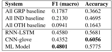
4.3 Sub-task C:

This task was the most challenging among the three tasks because of the small training data. The training data contains only 3876 tweets and the 3 sub-classes are unevenly distributed. First of

all, since this was a ternary classification task, we could only pursue a handful of machine learn-ing algorithms and secondly for neural network architectures, there is a paucity of huge dataset to train the model properly. We used 10% of training dataset for testing and validation pur-poses, while the rest used for training. We con-verted our text documents to a matrix of to-ken counts (CountVectorizer), then transformed a count matrix to a normalized tf-idf representation (tf-idf transformer). After that, we trained sev-eral classifiers from Scikit-Learn6 library. Now among the various classifiers, we built an en-semble (voting) classifier with top 5 models and found the best accuracy result for Logistic Re-gression. To make the vectorizer transformer-classifier easier to work with, we used Pipeline class in Scikit-Learn that behaves like a com-pound classifier. For RNN, the same previous sys-tem was used but with some alterations as change in labels and change in iterative conditions for output prediction as this was a ternary classifi-cation task. We obtained best results for Ma-chine Learning with Logistic Regression Classifier with 0.480057590252,0.577464788732 in terms of Macro-F1 and overall Accuracy respectively.

System F1 (macro) Accuracy

All GRP baseline 0.1787 0.3662

All IND baseline 0.2130 0.4695

All OTH baseline 0.0941 0.1643

RNN-LSTM 0.4580 0.5681

CNN-glove 0.4352 0.6056

ML Model 0.4801 0.5775

Table 5: Results for Sub-task C.

5 Observations

We noticed that both the F1(macro) and accuracy are high, in Sub-task A. This is probably due to relatively large size of training data. In sub-task B, we have found that, though the accuracy is op-timum, F1(macro) is surprisingly low. This is due to imbalanced dataset. Many classes have fewer samples to create robust models. This goes same for the sub-task C .

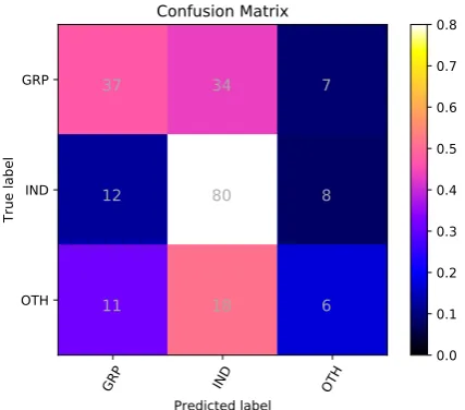
GRP IND _OTH

Predicted label GRP

IND

OTH

True label

37 34 7

12 80 8

11 18 6

Confusion Matrix

0.0 0.1 0.2 0.3 0.4 0.5 0.6 0.7 0.8

Figure 6: Confusion matrix of ML model for Sub-task C

6 Conclusions

In this paper, we have briefly described our sub-missions to SemEval2019 Task 6 on Identifica-tion and CategorizaIdentifica-tion of Offensive Language on Twitter data. Our systems ranked 21st out of 103 participants for Sub-task A, 50th out of 75 partic-ipants for Sub-task B and 47th out of 66 partici-pants for Sub-task C.Although our validation ac-curacy was high, the F1-score primarily dropped due to unequal distribution of opposite polarity data.

We could have made the system work better by training our model with additional tweets which we could have annotated manually. We could have also used Siamese Network to train our model, which has been generally used for image data.

References

Thomas Davidson, Dana Warmsley, Michael Macy, and Ingmar Weber. 2017. Automated Hate Speech Detection and the Problem of Offensive Language. InProceedings of ICWSM.

Mai ElSherief, Vivek Kulkarni, Dana Nguyen, William Yang Wang, and Elizabeth Belding. 2018. Hate Lingo: A Target-based Linguistic Analysis of Hate Speech in Social Media. arXiv preprint arXiv:1804.04257.

Darja Fiˇser, Tomaˇz Erjavec, and Nikola Ljubeˇsi´c. 2017. Legal Framework, Dataset and Annotation Schema for Socially Unacceptable On-line Discourse Prac-tices in Slovene. In Proceedings of the Workshop Workshop on Abusive Language Online (ALW), Van-couver, Canada.

Paula Fortuna and S´ergio Nunes. 2018. A Survey on Automatic Detection of Hate Speech in Text. ACM Computing Surveys (CSUR), 51(4):85.

Bj¨orn Gamb¨ack and Utpal Kumar Sikdar. 2017. Using Convolutional Neural Networks to Classify Hate-speech. In Proceedings of the First Workshop on Abusive Language Online, pages 85–90.

Ritesh Kumar, Atul Kr. Ojha, Shervin Malmasi, and Marcos Zampieri. 2018. Benchmarking Aggression Identification in Social Media. InProceedings of the First Workshop on Trolling, Aggression and Cyber-bulling (TRAC), Santa Fe, USA.

Shervin Malmasi and Marcos Zampieri. 2017. Detect-ing Hate Speech in Social Media. InProceedings of the International Conference Recent Advances in Natural Language Processing (RANLP), pages 467– 472.

Shervin Malmasi and Marcos Zampieri. 2018. Chal-lenges in Discriminating Profanity from Hate Speech. Journal of Experimental & Theoretical Ar-tificial Intelligence, 30:1–16.

Anna Schmidt and Michael Wiegand. 2017. A Sur-vey on Hate Speech Detection Using Natural Lan-guage Processing. InProceedings of the Fifth Inter-national Workshop on Natural Language Process-ing for Social Media. Association for Computational Linguistics, pages 1–10, Valencia, Spain.

Huei-Po Su, Chen-Jie Huang, Hao-Tsung Chang, and Chuan-Jie Lin. 2017. Rephrasing Profanity in Chi-nese Text. In Proceedings of the Workshop Work-shop on Abusive Language Online (ALW), Vancou-ver, Canada.

Zeerak Waseem, Thomas Davidson, Dana Warmsley, and Ingmar Weber. 2017. Understanding Abuse: A Typology of Abusive Language Detection Subtasks. In Proceedings of the First Workshop on Abusive Langauge Online.

Michael Wiegand, Melanie Siegel, and Josef Rup-penhofer. 2018. Overview of the GermEval 2018 Shared Task on the Identification of Offensive Lan-guage. InProceedings of GermEval.

Marcos Zampieri, Shervin Malmasi, Preslav Nakov, Sara Rosenthal, Noura Farra, and Ritesh Kumar. 2019a. Predicting the Type and Target of Offensive Posts in Social Media. InProceedings of NAACL.

Marcos Zampieri, Shervin Malmasi, Preslav Nakov, Sara Rosenthal, Noura Farra, and Ritesh Kumar. 2019b. SemEval-2019 Task 6: Identifying and Cat-egorizing Offensive Language in Social Media (Of-fensEval). InProceedings of The 13th International Workshop on Semantic Evaluation (SemEval).

Ziqi Zhang, David Robinson, and Jonathan Tepper. 2018. Detecting Hate Speech on Twitter Using a Convolution-GRU Based Deep Neural Network. In