Multi Relational Latent Semantic Analysis

Multi-Relational Latent Semantic Analysis

Kai-Wei Chang∗ University of Illinois Urbana, IL 61801, USA

[email protected]

Wen-tau Yih Christopher Meek Microsoft Research

Redmond, WA 98052, USA

{scottyih,meek}@microsoft.com

Abstract

We present Multi-Relational Latent Seman-tic Analysis (MRLSA) which generalizes La-tent Semantic Analysis (LSA). MRLSA pro-vides an elegant approach to combining mul-tiple relations between words by construct-ing a 3-way tensor. Similar to LSA, a low-rank approximation of the tensor is derived using a tensor decomposition. Each word in the vocabulary is thus represented by a vec-tor in the latent semantic space and each re-lation is captured by a latent square matrix. The degree of two words having a specific relation can then be measured through sim-ple linear algebraic operations. We demon-strate that by integrating multiple relations from both homogeneous and heterogeneous information sources, MRLSA achieves state-of-the-art performance on existing benchmark datasets for two relations,antonymyandis-a.

1 Introduction

Continuous semantic space representations have proven successful in a wide variety of NLP and IR applications, such as document clustering (Xu et al., 2003) and cross-lingual document retrieval (Dumais et al., 1997; Platt et al., 2010) at the document level and sentential semantics (Guo and Diab, 2012; Guo and Diab, 2013) and syntactic parsing (Socher et al., 2013) at the sentence level. Such representa-tions also play an important role in applicarepresenta-tions for lexical semantics, such as word sense disambigua-tion (Boyd-Graber et al., 2007), measuring word

∗

Work conducted while interning at Microsoft Research.

similarity (Deerwester et al., 1990) and relational similarity (Turney, 2006; Zhila et al., 2013; Mikolov et al., 2013). In many of these applications, La-tent Semantic Analysis (LSA) (Deerwester et al., 1990) has been widely used, serving as a fundamen-tal component or as a strong baseline.

LSA operates by mapping text objects, typically documents and words, to a latent semantic space. The proximity of the vectors in this space implies that the original text objects are semantically re-lated. However, one well-known limitation of LSA is that it is unable to differentiate fine-grained re-lations. For instance, when applied to lexical se-mantics, synonyms and antonyms may both be as-signed high similarity scores (Landauer and Laham, 1998; Landauer, 2002). Asymmetric relations like hyponyms and hypernyms also cannot be differenti-ated. Although there exists some recent work, such as PILSA which tries to overcome this weakness of LSA by introducing the notion of polarity (Yih et al., 2012). This extension, however, can only handle two opposing relations (e.g., synonyms and antonyms), leaving open the challenge of encoding multiple relations.

In this paper, we propose Multi-Relational Latent Semantic Analysis (MRLSA), which strictly gener-alizes LSA to incorporate information of multiple relations concurrently. Similar to LSA or PILSA when applied to lexical semantics, each word is still mapped to a vector in the latent space. However, when measuring whether two words have a specific relation (e.g., antonymy or is-a), the word vectors will be mapped to a new space according to the rela-tion where the degree of having this relarela-tion will be

judged by cosine similarity. The raw data construc-tion in MRLSA is straightforward and similar to the document-term matrix in LSA. However, instead of using one matrix to capture all relations, we extend the representation to a 3-way tensor. Each slice cor-responds to the document-term matrix in the original LSA design but for a specific relation. Analogous to LSA, the whole linear transformation mapping is de-rived through tensor decomposition, which provides a low-rank approximation of the original tensor. As a result, previously unseen relations between two words can be discovered, and the information en-coded in other relations can influence the construc-tion of the latent representaconstruc-tions, and thus poten-tially improves the overall quality. In addition, the information in different slices can come from het-erogeneous sources (conceptually similar to (Riedel et al., 2013)), which not only improves the model, but also extends the word coverage in a reliable way.

We provide empirical evidence that MRLSA is ef-fective using two different word relations:antonymy

andis-a. We use the benchmark GRE test of closest-opposites (Mohammad et al., 2008) to show that MRLSA performs comparably to PILSA, which was the pervious state-of-the-art approach on this prob-lem, when given the same amount of information. In addition, when other words and relations are avail-able, potentially from additional resources, MRLSA is able to outperform previous methods significantly. We use theis-arelation to demonstrate that MRLSA is capable of handling asymmetric relations. We take the list of word pairs from theClass-Inclusion

(i.e., is-a) relations in SemEval-2012 Task 2 (Jur-gens et al., 2012), and use our model to measure the degree of two words have this relation. The mea-sures derived from our model correlate with human judgement better than the best system that partici-pated in the task.

The rest of this paper is organized as follows. We first survey some related work in Section 2, followed by a more detailed description of LSA and PILSA in Section 3. Our proposed model, MRLSA, is pre-sented in Section 4. Section 5 presents our experi-mental results. Finally, Section 6 concludes the pa-per.

2 Related Work

MRLSA can be viewed as a model that derives gen-eral continuous spacerepresentationsfor capturing

lexical semantics, with the help oftensor decompo-sition techniques. We highlight some recent work related to our approach.

The most commonly used continuous space rep-resentation of text is arguably the vector space model (VSM) (Turney and Pantel, 2010). In this representation, each text object can be represented by a high-dimensional sparse vector, such as a term-vector or a document-vector that denotes the statistics of term occurrences (Salton et al., 1975) in a large corpus. The text can also be repre-sented by a low-dimensional dense vector derived by linear projection models like latent semantic analysis (LSA) (Deerwester et al., 1990), by dis-criminative learning methods like Siamese neural networks (Yih et al., 2011), recurrent neural net-works (Mikolov et al., 2013) and recursive neu-ral networks (Socher et al., 2011), or by graphical models such as probabilistic latent semantic anal-ysis (PLSA) (Hofmann, 1999) and latent Dirichlet allocation (LDA) (Blei et al., 2003). As a general-ization of LSA, MRLSA is also a linear projection model. However, while the words are represented by vectors as well, multiple relations between words are captured separately by matrices.

In the context of lexical semantics, VSMs provide a natural way of measuring semantic word related-ness by computing the distance between the cor-responding vectors, which has been a standard ap-proach (Agirre et al., 2009; Reisinger and Mooney, 2010; Yih and Qazvinian, 2012). These approaches do not apply directly to the problem of modeling other types of relations. Existing methods that do handle multiple relations often use a model com-bination scheme to integrate signals from various types of information sources. For instance, mor-phological variations discovered from the Google

pairs of words can be analogous, and then predicting it using a supervised model with features based on the frequencies of patterns in the corpus. Similarly, to measure whether two word pairs have the same relation, Zhila et al. (2013) proposed to combine het-erogeneous models, which achieved state-of-the-art performance. In comparison, MRLSA models mul-tiple lexical relations holistically. The degree that two words having a particular relation is estimated using the same linear function of the corresponding vectors and matrix.

Tensor decomposition generalizes matrix factor-ization and has been applied to several NLP applica-tions recently. For example, Cohen et al. (2013) pro-posed an approximation algorithm for PCFG pars-ing that relies on Kruskal decomposition. Van de Cruys et al. (2013) modeled the composition of subject-verb-object triples using Tucker decompo-sition, which results in a better similarity measure for transitive phrases. Similar to this construction but used in the community-based question answer-ing (CQA) scenario, Qiu et al. (2013) represented triples of question title, question content and answer as a tensor and applied 3-mode SVD to derive latent semantic representations for question matching. The construction of MRLSA bears some resemblance to the work that use tensors to capture triples. How-ever, our goal of modeling different relations for lex-ical semantics is very different from the intended us-age of tensor decomposition in the existing work.

3 Latent Semantic Analysis

Latent Semantic Analysis (LSA) (Deerwester et al., 1990) is a widely used continuous vector space model that maps words and documents into a low dimensional space. LSA consists of two main steps. First, taking a collection of ddocuments that con-tains words from a vocabulary list of sizen, it first constructs ad×ndocument-term matrixWto en-code the occurrence information of a word in a docu-ment. For instance, in its simplest form, the element Wi,j can be the term frequency of thej-th word in thei-th document. In practice, a weighting scheme that better captures the importance of a word in the document, such as TF×IDF (Salton et al., 1975), is often used instead. Notice that “document” here simply means a group of words and has been applied

W

X

=

U

V

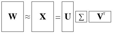
Figure 1: SVD applied to ad×ndocument-term ma-trixW. The rank-kapproximation,X, is the mul-tiplication of U, Σand VT, where U and V are

d×k andn×k orthonormal matrices andΣis a

k×kdiagonal matrix. The column vectors of VT multiplied by the singular valuesΣrepresent words in the latent semantic space.

to various texts including news articles, sentences and bags of words. Once the matrix is constructed, the second step is to apply singular value decom-position (SVD) toW in order to derive a low-rank approximation. To have a rank-kapproximation,X is the reconstruction matrix ofW, defined as

W≈X=UΣVT (1)

where the dimensions of U and V are d×k and

n×k, respectively, andΣis ak×kdiagonal ma-trix. In addition, the columns in U andV are or-thonormal and the elements in Σ are the singular values and are conventionally reverse-ordered. Fig-ure 1 illustrates this decomposition.

LSA can be used to compute the similarity be-tween two documents or two words in the latent space. For instance, to compare theu-th andv-th words in the vocabulary, one can compute the co-sine similarity of theu-th andv-th column vectors ofX, the reconstruction matrix ofW. In contrast to a direct lexical matching via the columns ofW, the similarity measure computed as a result of the SVD may have a nonzero similarity score even if these two words do not co-occur in any documents. This is due to the fact that those words can share some latent components.

joyfulness

gladden

sad 1

anger 1

-1

0 1

1

0

0 -1

0

1

0 0

-1

1

0 0

0

0

1 0

0

0

0 0

0

0

0

Figure 2: The matrix construction of PILSA. The vocabulary is{joy, gladden, sorrow, sadden, anger, emotion, feeling}and target words are{joyfulness, gladden, sad, anger}. For ease of presentation, we show the numbers with 0-1 values instead of TF×IDF scores. The polarity (i.e., sign) indicates whether the term in the vocabulary is a synonym or antonym of the target word.

which can be derived from the equations below.

XTX= (UΣVT)T(UΣVT)

=VΣUTUΣVT (Σis diagonal)

=VΣ2VT (Columns ofUare orthonormal)

= (ΣVT)T(ΣVT) (2)

Thus, the semantic relatedness between thei-th and

j-th words can be computed by cosine similarity1:

cos(X:,i,X:,j) (3)

When used to compare words, one well-known limitation of LSA is that the score captures the gen-eral notion of semantic similarity, and is unable to distinguish fine-grained word relations, such as antonyms (Landauer and Laham, 1998; Landauer, 2002). This is due to the fact that the raw matrix rep-resentation only records the occurrences of words in documents without knowing the specific relation be-tween the word and document. To address this issue, Yih et al. (2012) proposed a polarity inducing latent semantic analysis model recently, which we intro-duce next.

1_{Cosine similarity is equivalent to the inner product of the} normalized vectors.

3.1 Polarity Inducing Latent Semantic Analysis

In order to distinguish antonyms from synonyms, the polarity inducing LSA (PILSA) model (Yih et al., 2012) takes a thesaurus as input. Synonyms and antonyms of the same target word are grouped to-gether as a “document” and a document-term matrix is constructed accordingly as done in LSA. Because each word in a group belongs to either one of the two opposite relations,synonymyandantonymy, the po-larityinformation is induced by flipping the signs of antonyms. While the absolute value of each element in the matrix is still the same TF×IDF score, the elements that correspond to the antonyms become negative.

This design has an intriguing effect. When com-paring two words using the cosine similarity (or sim-ply inner product) of their corresponding column vectors in the matrix, the score of a synonym pair remains positive, but the score of an antonym pair becomes negative. Figure 2 illustrates this design using a simplified matrix as example.

Once the matrix is constructed, PILSA applies SVD as done in LSA, which generalizes the model to go beyond lexical matching. The sign of the co-sine score of the column vectors of any two words indicates whether they are close to synonyms or to antonyms and the absolute value reflects the degree of the relation. When all the column vectors are nor-malized to unit vectors, it can also be viewed as syn-onyms are clustered together and antsyn-onyms lie on the opposite sides of a unit sphere. Although PILSA successfully extends LSA to handle not just one sin-gle occurrencerelation, the extension is limited to encoding two opposing relations

4 Multi-Relational Latent Semantic Analysis

joyfulness gladden sad 1 anger 1 0 0 1 1 0 0 0 0 1 0 0 0 1 0 0 0 0 1 0 0 0 0 0 0 0 0

(a) Synonym layer

joyfulness gladden sad 0 anger 0 1 0 0 0 0 0 1 0 0 0 0 1 0 0 0 0 0 0 0 0 0 0 0 0 0 0

(b) Antonym layer

joyfulness gladden sad 0 anger 0 0 0 0 0 0 0 0 0 0 0 0 0 0 0 0 0 0 0 1 0 1 1 1 0 1 1

(c) Hypernym layer

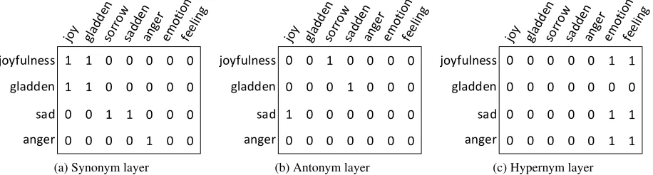
Figure 3: The three slices of MRLSA raw tensorWfor an example with vocabulary{joy, gladden, sorrow, sadden, anger, emotion, feeling}and target words{joyfulness, gladden, sad, anger}. Figures 3(a), 3(b), 3(c) show the matricesW_:,:,syn, W_:,:,ant, W_:,:,hyper, respectively. Rows represent documents (see definition in text), and columns represent words. For ease of presentation, we show numbers with 0-1 values instead of TF×IDF scores.

the Tucker decomposition, to the tensor.

4.1 Representing Multi-Relational Data in Tensors

A tensor is simply a multi-dimensional array. In this work, we use a 3-way tensor W to encode multi-ple word relations. An element of W is denoted by W_i,j,k using its indices, and W_:,:,k represents the k-th slice of W (a slice of a 3-way tensor is a matrix, obtained by fixing the third index). Fol-lowing (Kolda and Bader, 2009), a fiber of a ten-sorW_:,j,k is a vector, which is a high order analog of a matrix row or column.

When constructing the raw tensorW in MRLSA, each slice is analogous to the document-term ma-trix in LSA, but created based on the data of a par-ticular relation, such as synonyms. With a slight abuse of notation, we sometimes use the value rather than index when there is no confusion. For in-stance, W_{:,“word”,k} represents the fiber correspond-ing to the “word” in slice k, and W_:,:,syn refers to the slice that encodes the synonymy relation. Below we use an example to compare this construction to the raw matrix in PILSA, and discuss how it extends LSA.

Suppose we are interested in representing two re-lations, synonymy and antonymy. The raw tensor in MRLSA would then consist of two slices, W:,:,syn

andW_:,:,ant, to encode synonyms and antonyms of target words from a knowledge source (e.g., a the-saurus). Each row in W:,:,syn represents the

syn-onyms of a target word, and the corresponding row inW:,:,ant encodes its antonyms. Figures 3(a)

and 3(b) illustrate an example, where “joy”, ”glad-den” are synonyms of the target word “joyfulness” and “sorrow” is its antonym. Therefore, the values of the corresponding entries are 1. Notice that the matrixW0 = W_:,:,syn− W_:,:,ant is identical to the PILSA raw matrix. We can extend the construction above to enable MRLSA to utilize other semantic relations (e.g., hypernymy) by adding a slice cor-responding to each relation of interest. Fig. 3(c) demonstrates how to add another sliceW_:,:,hyper to the tensor for encoding hypernyms.

4.2 Tensor Decomposition

The MRLSA raw tensor encodes relations in one or more data resources, such as thesauri. However, the knowledge from a thesaurus is usually noisy and in-complete. In this section, we derive a low-rank ap-proximation of the tensor to generalize the knowl-edge. This step is analogous to the rank-k approxi-mation in LSA.

X

U

_V

G

T

V

=

W

(a) Tucker Tensor Decomposition

X

U

V

T

=

S

(b) Our Reformulation

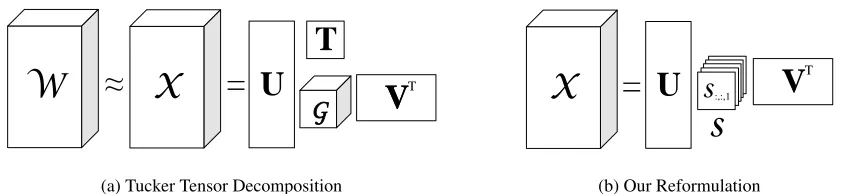
Figure 4: Fig. 4(a) illustrates the Tucker tensor decomposition method which factors a 3-way tensorW to three orthogonal matrices,U,V,T, and a core tensorG. We further apply an-mode matrix product on the core tensorG withT. Consequently, each slice of the resulted core tensorS (a square matrix) captures a semantic relation type, and each column ofVT _{is a vector representing a word.}

X ofWis defined by

W_i,j,k ≈ X_i,j,k

=

R1

X

r1=1

R2

X

r2=1

R3

X

r3=1

Gr1,r2,r3Ui,r1Vj,r2Tk,r3,

whereGis a core tensor with dimensionsR1×R2×

R3 and U,V,T are orthogonal matrices with

di-mensions d×R1, n ×R2, m× R3, respectively.

The rank parametersR1 ≤d, R2 ≤n, R3 ≤mare

given as input to the algorithm. In MRLSA,m(the number of relations) is usually small, whiledandn

are typically large (often in the scale of hundreds of thousands). Therefore, we chooseR1=R2 =τ,

τ d, nandR3=m, whereτis typically less than

1000.

To make the analogy to SVD clear, we rewrite the results of Tucker decomposition by performing an -mode matrix product over the core tensorGwith the matrixT. This produces a tensorSwhere each slice is a linear combination of the slices ofGwith coeffi-cients given byT(see (Kolda and Bader, 2009) for detail). That is, we have

S_:,:,k =

m X

t=1

Tt,kG:,:,t, ∀k.

An illustration is shown in Fig. 4(b), Then, a straightforward calculation shows that k-th slice of tensorW is approximated by

W_:,:,k ≈ X_:,:,k =US_:,:,kVT. (4) Comparing Eq. (4) to Eq. (1), one can observe that matricesU andVplay similar roles here, and

each slice of the core tensor S is analogous to Σ. However, the square matrix G_:,:,k is not necessary to be diagonal. As in SVD, the column vectors of G_:,:,kVT (capture both word and relation infor-mation) behave similarly to the column vectors of the original tensor sliceW:,:,k.

4.3 Measuring the Degrees of Word Relations

In principle, the raw information in the input ten-sorW can be used for computing lexical similarity using the cosine score between the column vectors for two words from the same slice of the tensor. To measure the degree of other relations, however, our approach requires one to specify apivotslice. The key role of the pivot slice is to expand the lexical coverage of the relation of interest to additional lexi-cal entries and, for this reason, the pivot slice should be chosen to capture the equivalence of the lexical entries. In this paper, we use the synonymy relation as our pivot slice. First we consider measuring the degree of a relationrelholding between thei-th and

j-th words using the raw tensor W, which can be computed as

cos W_:,i,syn,W_:,j,rel

. (5)

This measurement can be motivated from the logical rule: syn(wordi,target) ∧rel(target,wordj) →

rel(wordi,wordj), where the pivot relationsyn ex-pands the coverage of the relation of interestrel.

Turning to the use of the tensor decomposition, we use a similar derivation to Eq. (3), and measure the degree of relationrelbetween two words by

cos S:,:,synVi,T:,S:,:,relVTj,:

For instance, the degree of antonymy between “joy” and “sorrow” is measured by the co-sine similarity between the respective fibers

cos(X_{:,“joy”,syn},X_{:,“sorrow”,ant}). We can encode both

symmetric relations (e.g.,antonymyandsynonymy) and asymmetric relations (e.g., hypernymy and

hyponymy) in the same tensor representation. For a symmetric relation, we use bothcos(X_:,i,syn,X_:,j,rel)

andcos(X:,j,syn,X:,i,rel) and measure the degree of

a symmetric relation by the average of these two cosine similarity scores. However, for asymmetric relations, we use onlycos(X:,i,syn,X:,j,rel).

5 Experiments

We evaluate MRLSA on two tasks: answering the closest-opposite GRE questions and measuring de-grees of various class-inclusion (i.e.,is-a) relations. In both tasks, we design the experiments to empir-ically validate the following claims. When encod-ing two opposite relations from the same source, MRLSA performs comparably to PILSA. However, MRLSA generalizes LSA to model multiple rela-tions, which could be obtained from both homoge-neous and heterogehomoge-neous data sources. As a result, the performance of a target task can be further im-proved.

5.1 Experimental Setup

We construct the raw tensors to encode a particular relation in each slice based on two data sources.

Encarta The Encarta thesaurus is developed by Bloomsbury Publishing Plc2. For each target word, it provides a list of synonyms and antonyms. We use the same version of the thesaurus as in (Yih et al., 2012), which contains about 47k words and a vocabulary list of approximately 50k words.

WordNet We use four types of relations from WordNet: synonymy, antonymy, hypernymy and hyponymy. The number of target words and the size of the vocabulary in our version are 117,791 and 149,400, respectively. WordNet has better vo-cabulary coverage, but fewer antonym pairs. For instance, the WordNet antonym slice contains only 46,945 nonzero entries, while the Encarta antonym slice has 129,733.

2

http://www.bloomsbury.com

We apply a memory-efficient Tucker decomposi-tion algorithm (Kolda and Sun, 2008) implemented intensor toolbox v2.5(Bader et al., 2012)3to factor the tensor. The largest tensor considered in this pa-per can be decomposed in about 3 hours using less than 4GB of memory with a commodity PC.

5.2 Answering GRE Antonym Questions

The first task is to answer the closest-opposite ques-tions from the GRE test provided by Mohammad et al. (2008)4. Each question in this test consists of a target word and five candidate words, where the goal is to pick the candidate word that has the most opposite meaning to the target word. In order to have a fair comparison, we use the same data split as in (Mohammad et al., 2008), with 162 questions used for the development set and 950 for test. Fol-lowing (Mohammad et al., 2008; Yih et al., 2012), we report the results in precision (accuracy of the questions that the system attempts to answer), re-call (percentage of the questions answered correctly over all questions) and F1 (the harmonic mean of

precision and recall).

We tune two sets of parameters using the devel-opment set: (1) the rank parameterτ in the tensor decomposition and (2) the scaling factors of differ-ent slices of the tensor. The rank parameter spec-ifies the number of dimensions of the latent space. In the experiments, We pick the best value ofτ from {100,200,300,500,750,1000}. The scaling factors adjust the values of each slice of the tensor. The el-ements of each slice are multiplied by the scaling factor before factorization. This is important be-cause Tucker decomposition minimizes the recon-struction error (the Frobenius norm of the residual tensor). As a result, the slice with a larger range of values becomes more influential toUandV. In this work, we fixW:,:,ant, and search for the scaling

fac-tor ofW_:,:,syn in {0.25,0.5,1,2,4} and the factors

ofW:,:,hyperandW:,:,hypoin{0.0625,0.125,0.25}.

Table 1 summarizes the results of training

3

http://www.sandia.gov/˜tgkolda/

TensorToolbox. The Tucker decomposition involves performing SVD on a large matrix. We modify the MATLAB code oftensor toolboxto use the built-insvdfunction instead ofsvds. This modification reduces both the running time and memory usage.

4

Dev. Set Test Set Prec. Rec. F1 Prec. Rec. F1

WordNet Lookup 0.40 0.40 0.40 0.42 0.41 0.42 WordNet RawTensor 0.42 0.41 0.42 0.42 0.41 0.42 WordNet PILSA 0.63 0.62 0.62 0.60 0.60 0.60 WordNet MRLSA:Syn+Ant 0.63 0.62 0.62 0.59 0.58 0.59 WordNet MRLSA:4-layers 0.66 0.65 0.65 0.61 0.59 0.60 Encarta Lookup 0.65 0.61 0.63 0.61 0.56 0.59 Encarta RawTensor 0.67 0.64 0.65 0.62 0.57 0.59 Encarta PILSA 0.86 0.81 0.84 0.81 0.74 0.77 Encarta MRLSA:Syn+Ant 0.87 0.82 0.84 0.82 0.74 0.78 MRLSA:WordNet+Encarta 0.88 0.85 0.87 0.81 0.77 0.79

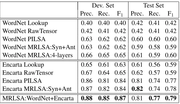
Table 1: GRE antonym test results of models based on Encarta and WordNet data in precision, recall and F1.

RawTensor evaluates the performance of the tensor with 2 slices encoding synonyms and antonyms be-fore decomposition (see Eq. (5)), which is comparable to checking the original data directly (Lookup). MRLSA:Syn+Ant applies Tucker decomposition to the raw tensor and measures the degree of antonymy using Eq. (6). The result is similar to that of PILSA (see Sec. 3.1). MRLSA:4-layers adds hypernyms and hyponyms from WordNet; MRLSA:WordNet+Encarta consists of synonyms/antonyms from Encarta and hy-pernyms/hyponyms from WordNet, where the target words are aligned using the synonymy relations. Both models demonstrate the advantage of encoding more relations, from either the same or different resources.

MRLSA using two different corpora, Encarta and WordNet. The performance of the MRLSA raw tensor is close to that of looking up the thesaurus. This indicates the tensor representation is able to capture the word relations explicitly described in the thesaurus. After conducting tensor decomposi-tion, MRLSA:Syn+Ant achieves similar results to PILSA. This confirms our claim that when giv-ing the same among of information, MRLSA per-forms at least comparably to PILSA. However, the true power of MRLSA is its ability to incorpo-rate other semantic relations to boost the perfor-mance of the target task. For example, when we add the hypernymy and hyponymy relations to the tensor, these class-inclusion relations provide a weak signal to help resolve antonymy. We sus-pect that this is due to the fact that antonyms typ-ically share the same properties but only have the opposite meaning on one particular semantic di-mension. For instance, the antonyms “sadness” and “happiness” are different forms of emotion. When two words are hyponyms of a target word, the likelihood that they are antonyms should thus be increased. We show that the target relations and these auxiliary semantic relations can be

col-lected from the same data source (e.g., WordNet MRLSA:4-layers) or from multiple, heterogeneous sources (e.g., MRLSA:WordNET+Encarta). In both cases, the performance of the model improves as more relations are incorporated. Moreover, our ex-periments show that adding the hypernym and hy-ponym layers from WordNet improves modeling antonym relations based on the Encarta thesaurus. This suggests that the weak signal from a resource with a large vocabulary (e.g., WordNet) can help predict relations between out-of-vocabulary words and thus improve the recall.

To better understand the model, we examine the top antonyms for three question words from the GRE test. The lists below show antonyms and their MRLSA scores for each of the GRE question words as determined by the MRLSA:WordNET+Encarta model. Antonyms that can be found directly in the Encarta thesaurus are in italics.

inanimate alive(0.91), living (0.90), bodily(0.90), in-the-flesh (0.89),incarnate(0.89)

alleviate exacerbate (0.68), make-worse (0.67), in-flame (0.66), amplify (0.65), stir-up (0.64)

relish detest (0.33), abhor (0.33), abominate (0.33), de-spise (0.33), loathe (0.31)

Dev. Test

1a (Taxonomic) 1b (Functional) 1c (Singular) 1d (Plural) Avg.

WordNet Lookup 52.9 34.5 41.4 34.3 36.7

WordNet RawTensor 51.0 38.3 50.0 42.1 43.5

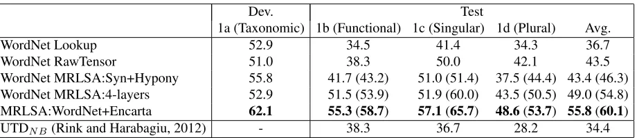
WordNet MRLSA:Syn+Hypony 55.8 41.7 (43.2) 51.0 (51.4) 37.5 (44.4) 43.4 (46.3) WordNet MRLSA:4-layers 52.9 51.5 (53.9) 51.9 (60.0) 43.5 (50.5) 49.0 (54.8) MRLSA:WordNet+Encarta 62.1 55.3(58.7) 57.1(65.7) 48.6(53.7) 55.8(60.1) UTDN B(Rink and Harabagiu, 2012) - 38.3 36.7 28.2 34.4

Table 2: Results of measuring the class-inclusion (is-a) relations in MaxDiff accuracy (see text for de-tail). RawTensor has synonym and hyponym slices and measures the degree ofis-arelation using Eq. (5). MRLSA:Syn+Hypo factors the raw tensor and judges the relation by Eq. (6). The constructions of MRLSA:4-layers and MRLSA:WordNet+Encarta are the same as in Sec. 5.2 (see the caption of Table 1 for detail). For MRLSA models, numbers shown in the parentheses are the results when parameters are tuned using the test sets. UTDN B is the results of the best performing system in SemEval-2012 Task 2.

only preserves the antonyms in the thesaurus, but also discovers additional ones, such as exacerbate

andinflamefor “alleviate”. Another interesting find-ing is that while the scores are useful in rankfind-ing the candidate words, they might not be comparable across different question words. This could be an issue for some applications, which need to make a binary decision on whether two words are antonyms.

5.3 Measuring degrees ofIs-Arelations

We evaluate MRLSA using the class-inclusion por-tion of SemEval-2012 Task 2 data (Jurgens et al., 2012). Here the goal is to measure the degree of two words having the is-a relation. Five an-notated datasets are provided for different subcate-gories of this relation: 1a-taxonomic, 1b-functional, 1c-singular, 1d-plural, 1e-class individual. We omit 1e because it focuses on real world entities (e.g., queen:Elizabeth, river:Nile), which are not included in WordNet.

Each dataset contains about 100 questions based on approximately 40 word pairs. The question con-sists of 4 randomly chosen word pairs and asks the best and worst pairs that exemplify the specificis-a

relation. The performance is measured by the av-erage prediction accuracy, also called the MaxDiff accuracy (Louviere and Woodworth, 1991).

Because the questions are generated from the same set of word pairs, these questions are not mutu-ally independent. Therefore, it is not proper to split the data of each subcategory into the development and test sets. Alternatively, we follow the setting

of SemEval-2012 Task 2 and use the first subcat-egory (1a-taxonomy) to tune the model and eval-uate its performance based on the results on other datasets. Since the models are tuned and tested on different types of subcategories, they might not be the optimal ones when evaluated on the test sets. Therefore, we show results using the best parame-ters tuned on the development set and those tuned on the test set, where the latter suggests a performance upper-bound. Besides the rank parameter, we tune the scaling factors of the synonym, hypernym and hyponym slices from{4, 16, 64}. The scaling factor of the antonym slice is fixed to 1.

outper-forms the best system participated in the SemEval-2012 task with a large margin, with a difference of 21.4 in MaxDiff accuracy.

Next we examine the top words that have the is-arelation relative to three question words from the task. The lists below show the hyponyms and their respective MRLSA scores for each of the question words as determined by MRLSA:4-layers.

bird ostrich (0.75), gamecock (0.75), nighthawk (0.75), amazon (0.74), parrot (0.74)

automobile minivan (0.48), wagon (0.48), taxi (0.46), minicab (0.45), gypsy cab (0.45)

vegetable buttercrunch (0.61), yellow turnip (0.61), ro-maine (0.61), chipotle (0.61), chilli (0.61)

Although the model in general does a good job finding hyponyms, we observe that some suggested words, such as buttercrunch (a mild lettuce) vs. “vegetable”, do not seem intuitive (e.g., compared to

carrot). Having one additional slice to capture the general term co-occurrence relation may help im-prove the model in this respect.

6 Conclusions

In this paper, we propose Multi-Relational Latent Semantic Analysis (MRLSA) which generalizes La-tent Semantic Analysis (LSA) for lexical seman-tics. MRLSA models multiple word relations by leveraging a 3-way tensor, where each slice cap-tures one particular relation. A low-rank approx-imation of the tensor is then derived using a ten-sor decomposition. Consequently, words in the vo-cabulary are represented by vectors in the latent se-mantic space, and each relation is captured by a latent square matrix. Given two words, MRLSA not only can measure their degree of having a spe-cific relation, but also can discover unknown rela-tions between them. These advantages have been demonstrated in our experiments. By encoding re-lations from both homogeneous or heterogeneous data sources, MRLSA achieves state-of-the-art per-formance on existing benchmark datasets for two re-lations,antonymyandis-a.

For future work, we plan to explore directions that aim for improving both the quality and word cover-age of the model. For instance, the knowledge en-coded by MRLSA can be enriched by adding more relations from a variety of linguistic resources, in-cluding the co-occurrence relations from large

cor-pora. On model refinement, we notice that MRLSA can be viewed as a 3-layer neural network without applying the sigmoid function. Following the strat-egy of using Siamese neural networks to enhance PILSA (Yih et al., 2012), training MRLSA with a multi-task discriminative learning setting can be a promising approach as well.

Acknowledgments

We thank Geoff Zweig for valuable discussions and the anonymous reviewers for their comments.

References

E. Agirre, E. Alfonseca, K. Hall, J. Kravalova, M. Pas¸ca and A. Soroa. 2009. A study on similarity and re-latedness using distributional and WordNet-based ap-proaches. InNAACL ’09, pages 19–27.

Brett W. Bader, Tamara G. Kolda, et al. 2012. Matlab tensor toolbox version 2.5. Available online, January. David M. Blei, Andrew Y. Ng, Michael I. Jordan, and

John Lafferty. 2003. Latent dirichlet allocation. Jour-nal of Machine Learning Research, 3:993–1022. Jordan L Boyd-Graber, David M Blei, and Xiaojin Zhu.

2007. A topic model for word sense disambiguation. InEMNLP-CoNLL, pages 1024–1033.

Shay B. Cohen, Giorgio Satta, and Michael Collins. 2013. Approximate PCFG parsing using tensor de-composition. InNAACL-HLT 2013, pages 487–496. S. Deerwester, S. Dumais, G. Furnas, T. Landauer, and

R. Harshman. 1990. Indexing by latent semantic anal-ysis. Journal of the American Society for Information Science, 41(96).

S. Dumais, T. Letsche, M. Littman, and T. Landauer. 1997. Automatic cross-language retrieval using latent semantic indexing. InAAAI-97 Spring Symposium Se-ries: Cross-Language Text and Speech Retrieval. Weiwei Guo and Mona Diab. 2012. Modeling sentences

in the latent space. InACL 2012, pages 864–872. Weiwei Guo and Mona Diab. 2013. Improving lexical

semantics for sentential semantics: Modeling selec-tional preference and similar words in a latent variable model. InNAACL-HLT 2013, pages 739–745. Thomas Hofmann. 1999. Probabilistic latent semantic

analysis. In Proceedings of Uncertainty in Artificial Intelligence, pages 289–296.

Tamara G. Kolda and Brett W. Bader. 2009. Ten-sor decompositions and applications. SIAM Review, 51(3):455–500, September.

Tamara G. Kolda and Jimeng Sun. 2008. Scalable ten-sor decompositions for multi-aspect data mining. In ICDM 2008, pages 363–372.

T. Landauer and D. Laham. 1998. Learning human-like knowledge by singular value decomposition: A progress report. InNIPS 1998.

T. Landauer. 2002. On the computational basis of learn-ing and cognition: Arguments from lsa. Psychology of Learning and Motivation, 41:43–84.

Jordan J. Louviere and G. G. Woodworth. 1991. Best-worst scaling: A model for the largest difference judg-ments. Technical report, University of Alberta. Tomas Mikolov, Wen-tau Yih, and Geoffrey Zweig.

2013. Linguistic regularities in continuous space word representations. InNAACL-HLT 2013.

Saif Mohammad, Bonnie Dorr, and Graeme Hirst. 2008. Computing word pair antonymy. InEmpirical Meth-ods in Natural Language Processing (EMNLP). John Platt, Kristina Toutanova, and Wen-tau Yih. 2010.

Translingual document representations from discrimi-native projections. InProceedings of EMNLP, pages 251–261.

Xipeng Qiu, Le Tian, and Xuanjing Huang. 2013. Latent semantic tensor indexing for community-based ques-tion answering. In Proceedings of the 51st Annual Meeting of the Association for Computational Linguis-tics (Volume 2: Short Papers), pages 434–439, Sofia, Bulgaria, August. Association for Computational Lin-guistics.

Joseph Reisinger and Raymond J. Mooney. 2010. Multi-prototype vector-space models of word meaning. In Proceedings of HLT-NAACL, pages 109–117.

Sebastian Riedel, Limin Yao, Andrew McCallum, and Benjamin M. Marlin. 2013. Relation extraction with matrix factorization and universal schemas. In NAACL-HLT 2013, pages 74–84.

Bryan Rink and Sanda Harabagiu. 2012. UTD: Deter-mining relational similarity using lexical patterns. In Proceedings of the Sixth International Workshop on Semantic Evaluation (SemEval 2012), pages 413–418, Montr´eal, Canada, 7-8 June. Association for Compu-tational Linguistics.

G. Salton, A. Wong, and C. S. Yang. 1975. A Vector Space Model for Automatic Indexing. Communica-tions of the ACM, 18(11).

Richard Socher, Cliff Chiung-Yu Lin, Andrew Y. Ng, and Christopher D. Manning. 2011. Parsing natural scenes and natural language with recursive neural net-works. InICML ’11.

Richard Socher, John Bauer, Christopher D. Manning, and Andrew Y. Ng. 2013. Parsing with compositional vector grammars. InAnnual Meeting of the Associa-tion for ComputaAssocia-tional Linguistics (ACL).

Ledyard R Tucker. 1966. Some mathematical notes on three-mode factor analysis. Psychometrika, 31(3):279–311.

Peter D. Turney and Patrick Pantel. 2010. From fre-quency to meaning: Vector space models of semantics. Journal of Artificial Intelligence Research, 37(1):141– 188.

P. D. Turney. 2006. Similarity of semantic relations. Computational Linguistics, 32(3):379–416.

Peter Turney. 2008. A uniform approach to analo-gies, synonyms, antonyms, and associations. In In-ternational Conference on Computational Linguistics (COLING).

Tim Van de Cruys, Thierry Poibeau, and Anna Korho-nen. 2013. A tensor-based factorization model of se-mantic compositionality. InProceedings of the 2013 Conference of the North American Chapter of the As-sociation for Computational Linguistics: Human Lan-guage Technologies, pages 1142–1151, Atlanta, Geor-gia, June. Association for Computational Linguistics. Wei Xu, Xin Liu, and Yihong Gong. 2003. Document

clustering based on non-negative matrix factorization. InProceedings of the 26th annual international ACM SIGIR conference on Research and development in in-formaion retrieval, pages 267–273, New York, NY, USA. ACM.

Wen-tau Yih and Vahed Qazvinian. 2012. Measur-ing word relatedness usMeasur-ing heterogeneous vector space models. InProceedings of NAACL-HLT, pages 616– 620, Montr´eal, Canada, June.

Wen-tau Yih, Kristina Toutanova, John C. Platt, and Christopher Meek. 2011. Learning discriminative projections for text similarity measures. In Proceed-ings of the Fifteenth Conference on Computational Natural Language Learning, pages 247–256, Portland, Oregon, USA, June. Association for Computational Linguistics.

Wen-tau Yih, Geoffrey Zweig, and John Platt. 2012. Po-larity inducing latent semantic analysis. In Proceed-ings of NAACL-HLT, pages 1212–1222, Jeju Island, Korea, July.