US YIELD FORECASTING USING CROP CONDITION RATINGS
BY
FERNANDA de BARROS DIAS
THESIS
Submitted in partial fulfillment of the requirements
for the degree of Master of Science in Agricultural and Applied Economics in the Graduate College of the
University of Illinois at Urbana-Champaign, 2017
Urbana, Illinois Master’s Committee:
Professor Scott Irwin, Chair Professor Gary Schnitkey Professor Emeritus Darrel Good
ii
ABSTRACT
This thesis studied the relationship between US average yield for the five main crops grown in the United States, corn, soybeans, upland cotton, winter wheat, and spring wheat, and crop condition ratings from 1986 to 2015. Three statistical models were tested, the first one including all categories of condition ratings, a trend, and no intercept. The second model addresses the issue of abandoned acres following the ideas of Fackler & Norwood and included all categories less the Very Poor category, a trend, and no intercept. The last model investigated is the sum of Good and Excellent categories, a trend, and intercept. The models were used to forecast US yield out-of-sample as an alternative to the benchmark forecast WASDE. Major findings include: 1) crop condition ratings will not be a good predictor of US average yield if there is an increase in the WASDE yield forecasting and the conditions are not aligned accordingly, 2) when weather becomes an issue these models perform very well compared to WASDE as it was the case in 2012, 3) the models are a good forecast beating the USDA
WASDE in almost every instance for the trend-yield months, 4) almost in every instance the best performing model did not use USDA’s original ratings, which implies that the corrections made to the data are rational, 5) except for soybeans and spring wheat, the WASDE survey-yield months are a better forecast than the statistical models developed in this thesis given the nature of the commodities and USDA’s superior method, 6) weighting by production instead of planted acres becomes particularly important when there is a wide range of yield variability between states like it is the case for corn and winter wheat, 7) correction for bias becomes particularly important the more the crop is sensitive to adverse events that affect yield during its reproduction stage.
iii TABLES OF CONTENTS LIST OF TABLES………...vii LIST OF FIGURES………...x 1. INTRODUCTION………...1 1.1 Background………....1 1.2 Objectives ……….…3
1.3 Data and Method………..…..4
1.4 Overview………..……..5
2. REVIEW OF THE LITERATURE……….6
2.1 Introduction………....6
2.2 Agronomy Theory……….….6
2.3 Remote Sensing ………..10
2.4 Crop Weather………..….13
2.5 Crop Condition Models………...…16
2.6 Summary………..24
3. DATA………28
3.1 Introduction………..28
3.2 The Crop Progress and Condition Report………....28
3.3 The Crop Progress and Condition Report Production……….…29
iv
3.5Descriptive Analysis of the Data…….………...……….……32
3.5.1 Corn………....34 3.5.2 Soybeans………....36 3.5.3 Upland Cotton………..…..38 3.5.4 Winter Wheat………...………..39 3.5.5 Spring Wheat……….………....40 3.5.6 Yields………...…….….41 3.6Summary………..………....42
4. MODELS AND IN-SAMPLE ANALYSIS …….………..…….….43
4.1 Introduction………..43
4.2 Conceptual Framework………....43
4.3 Results for Corn………..….47
4.4 Results for Soybeans………48
4.5 Results for Upland Cotton………..….49
4.6 Results for Winter Wheat………...…50
4.7 Results for Spring Wheat……….51
4.8 Summary………..……52
5. A YIELD FORECASTING COMPETITION……….…..…………...55
5.1 Introduction………..…55
5.2 Development of the Yield Prediction Competition……….55
5.2.1 Original Crop Condition Ratings……….…….55
v
5.2.3 Production Weights………..…….56
5.3 Evaluation Standards……….……..57
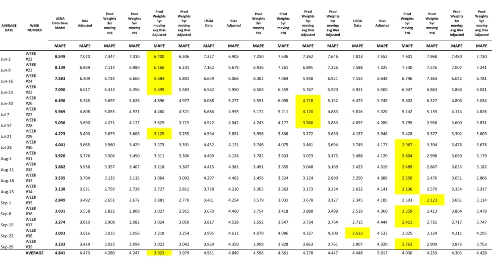
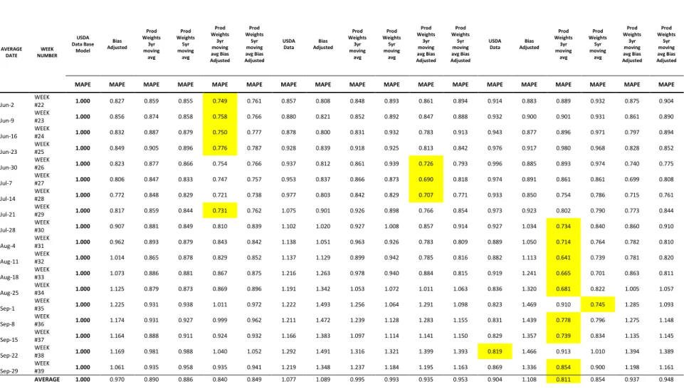
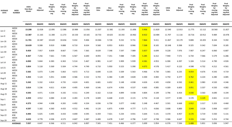
5.4 Forecasting Results………..58
5.4.1 Corn Yield Forecasts Results Model Comparison………....59
5.4.2 Corn Yield Forecasts Results Best Performing Model vs. WASDE………61
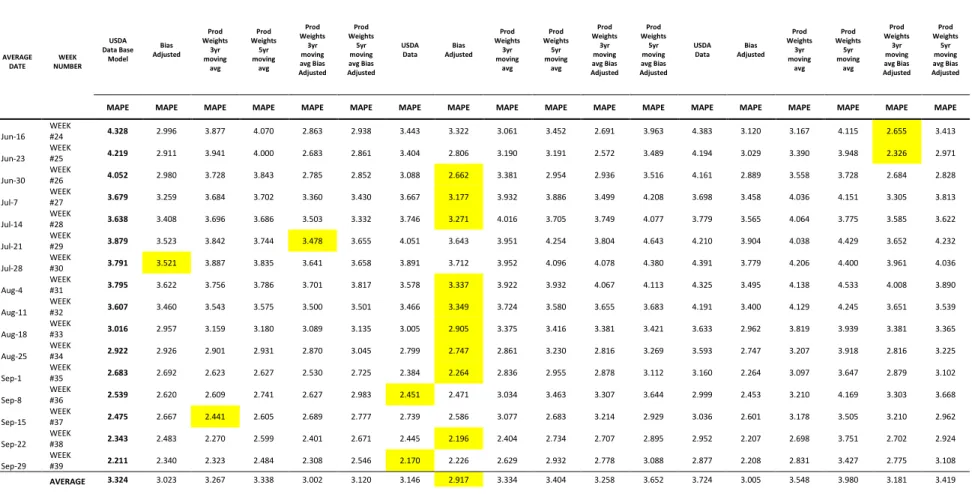
5.4.3 Soybean Yield Forecasts Results Model Comparison…………...62
5.4.4 Soybean Yield Forecasts Results Best Performing Model vs. WASDE…..63
5.4.5 Upland Cotton Yield Forecasts Results Model Comparison………63
5.4.6 Upland Cotton Yield Forecasts Results Best Performing Model vs. WASDE……….64
5.4.7 Winter Wheat Yield Forecasts Results Model Comparison……….65
5.4.8 Winter Wheat Yield Forecasts Results Best Performing Model vs. WASDE……….66
5.4.9 Spring Wheat Yield Forecasts Results Model Comparison…….………….66
5.4.10 Spring Wheat Yield Forecasts Results Best Performing Model vs. WASDE……….67
5.5 Summary……….……….68
6. CONCLUSION……….………..69
vi
6.2 Summary of Findings………...…70
6.3 Future Work and Concluding Remarks………..….72
FIGURES AND TABLES………...75
vii
LIST OF TABLES
Table 1. Corn- Mean and St. Deviation Difference between the last week and other week’s
ratings during the year per category………...80
Table 2. Soybeans- Mean and St. Deviation Difference between the last week and other week’s ratings during the year per category………...83
Table 3. Cotton, Upland- Mean and St. Deviation Difference between the last week and other week’s ratings during the year per category………..86
Table 4. Winter Wheat- Mean and St. Deviation Difference between the last week and other week’s ratings during the year per category………..…89
Table 5. Spring Wheat- Mean and St. Deviation Difference between the last week and other week’s ratings during the year per category………..…92
Table 6. National Level Coefficients Estimates for Corn, 1986-2015………....130
Table 7. National Level Coefficients Estimates for Soybeans, 1986-2015………...131
Table 8. National Level Coefficients Estimates for Cotton Upland, 1986-2015……….132
Table 9. National Level Coefficients Estimates for Winter Wheat, 1986-2015………..…133
Table 10. National Level Coefficients Estimates for Spring Wheat, 1986-2015…………...….134
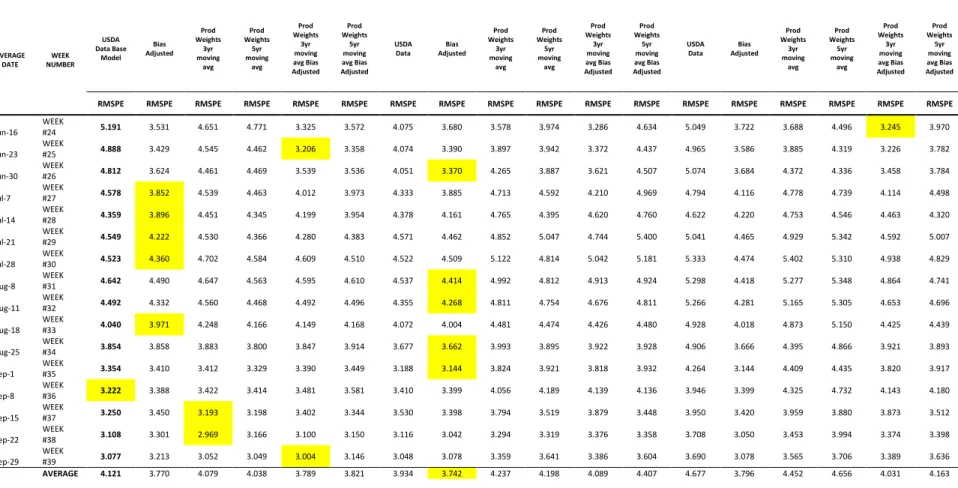
Table 11. Corn Yield Forecast Weekly Errors 2006-2015………..135
viii
Table 13. Corn Yield Forecast Weekly Errors 2006-2015………..137
Table 14. Corn Yield Forecast Weekly Errors 2006-2015 RMSPE RATIO………...138
Table 15. Soybean Yield Forecast Weekly Errors 2006-2015………139
Table 16. Soybean Yield Forecast Weekly Errors 2006-2015 MAPE RATIO………...…140
Table 17. Soybean Yield Forecast Weekly Errors 2006-2015………....141
Table 18. Soybean Yield Forecast Weekly Errors 2006-2015 RMSPE RATIO………...142
Table 19. Cotton, Upland Yield Forecast Weekly Errors 2006-2015………..143
Table 20. Cotton, Upland Yield Forecast Weekly Errors 2006-2015 MAPE RATIO………....144
Table 21. Cotton, Upland Yield Forecast Weekly Errors 2006-2015………..145
Table 22. Cotton, Upland Yield Forecast Weekly Errors 2006-2015 RMSPE RATIO………..146
Table 23. Winter Wheat Yield Forecast Weekly Errors 2006-2015………..…..147
Table 24. Winter Wheat Yield Forecast Weekly Errors 2006-2015 MAPE RATIO……….….148
Table 25. Winter Wheat Yield Forecast Weekly Errors 2006-2015………....149
Table 26. Winter Wheat Yield Forecast Weekly Errors 2006-2015 RMSPE RATIO…………150
Table 27. Spring Wheat Yield Forecast Weekly Errors 2006-2015………....151
Table 28. Spring Wheat Yield Forecast Weekly Errors 2006-2015 MAPE RATIO………..….152
Table 29. Spring Wheat Yield Forecast Weekly Errors 2006-2015…….………...153
ix
Table 31. Corn Yield Forecast Error Comparison 2006-2015………...…..155
Table 32. Corn Yield Forecast Error Comparison 2006-2015………...156
Table 33.Soybean Yield Forecast Error Comparison 2006-2015………....157
Table 34. Soybean Yield Forecast Error Comparison 2006-2015………...…158
Table 35. Cotton, Upland Yield Forecast Error Comparison 2006-2015………....159
Table 36. Cotton, Upland Yield Forecast Error Comparison 2006-2015………160
Table 37. Winter Wheat Yield Forecast Error Comparison 2006-2015………..161
Table 38. Winter Wheat Yield Forecast Error Comparison 2006-2015………..…162
Table 39. Spring Wheat Yield Forecast Error Comparison 2006-2015……….…..163
x
LIST OF FIGURES
Figure 1. Corn- Condition Ratings Mean for Each Category for Years 1986 to 2015, Beginning, Middle, and End of the Season………. 75 Figure 2. Soybeans- Condition Ratings Mean for Each Category for Years 1986 to 2015,
Beginning, Middle, and End of the Season………76 Figure 3. Cotton, Upland- Condition Ratings Mean for Each Category for Years 1986 to 2015, Beginning, Middle, and End of the Season………77 Figure 4. Winter Wheat- Condition Ratings Mean for Each Category for Years 1986 to 2015, Beginning, Middle, and End of the Season………78 Figure 5. Spring Wheat- Condition Ratings Mean for Each Category for Years 1986 to 2015, Beginning, Middle, and End of the Season………79 Figure 6. Corn- Mean Difference of Ratings for Each Category per Week for Years 1986 to 2015, June 2-39………...…...95 Figure 7. Soybeans- Mean Difference of Ratings for Each Category per Week for Years 1986 to 2015, June 16-39……….…...98 Figure 8. Cotton, Upland- Mean Difference of Ratings for Each Category per Week for Years 1986 to 2015, June 16-39……….…101 Figure 9. Winter Wheat- Mean Difference of Ratings for Each Category per Week for Years 1986 to 2015, April 7-25……….….…104
xi Figure 10. Spring Wheat- Mean Difference of Ratings for Each Category per Week for Years
1986 to 2015, June 9-31………...…107
Figure 11. Corn- Standard Deviation of Ratings per Week, 1986-2015……….110
Figure 12. Soybeans- Standard Deviation of Ratings per Week, 1986-2015………..113
Figure 13. Cotton, Upland- Standard Deviation of Ratings per Week, 1986-2015……….116
Figure 14. Winter Wheat- Standard Deviation of Ratings per Week, 1986-2015………...119
Figure 15. Spring Wheat- Standard Deviation of Ratings per Week, 1986-2015………...122
Figure 16. Average U.S Corn Yield, 1986-2015……….125
Figure 17. Average U.S Soybean Yield, 1986-2015………...126
Figure 18. Average U.S Cotton, Upland Yield, 1986-2015……….127
Figure 19. Average U.S Winter Wheat Yield, 1986-2015………...128
1
1. INTRODUCTION
1.1Background
Crop yield forecasting is of main concern for market participants from farmers to commercial trading companies, such as large agricultural companies, and non-commercial trading companies, such as hedge funds. Early season production forecast is key to price discovery mechanism for those billion dollar crops. Yield forecast has major impact on
positions taken in the market according to what is the anticipated supply of crops and the given demand. Not many studies have truly forecasted yield out of sample and compared to a
benchmark forecast such as the one provided by the USDA World Agricultural Supply and
Demand Estimates (WASDE).
Furthermore, crop condition ratings are the most widely used indicator of yield potential by market participants throughout the growing season of crops, however, little research has been done using the ratings. Lehecka (2014) investigated the informational value of the crop condition ratings during report release days and non-report release days finding significant differences in return variabilities between the two proving the impact of the weekly release of crop condition ratings has on market participants. Only two previous studies, Kruse & Smith and Fackler & Norwood, have analyzed crop condition ratings as a forecasting tool but at the time of their research there was not enough observations to make an out-of-sample forecast. The estimates in both papers were in-sample, therefore, not aligned with the USDA WASDE, which is a true forecast. This thesis aims to fill the gap in the literature of using crop condition ratings to make out of sample yield forecast of the main commodities grown in the United States.
Other lines of research have mainly focused on agronomy simulation models that
2 model. Furthermore, these models are usually not made to be applicable at a large regional scale making it problematic to obtain a forecast of yield on the national or state level. Remote sensing imagery of crops is another method that has been applied to forecast yield but the technique needs improvement in its spatial resolution and cost-effectiveness since the technique is not widely available to a wide range of market participants. The hybrid of those two facets of research showed improvement over the use of only one or another but still remain ineffective in conveying useful information for market participants’ decision making in a timely manner.
Empirical studies, on the other hand, make use of information that incorporates the
determinants of crop yield in a broad sense. For instance, the USDA crop condition ratings data used in this thesis conveys information about how the crops are developing responding to a variety of events throughout the growing season such as weather, pests and diseases, and it is reported every week from April to November, as mentioned before, being the most widely used indicator of yield potential.
As mentioned before, this thesis focuses mainly on the ideas developed by Kruse and Smith (1994) and Fackler and Norwood (1999). Kruse and Smith associated a given set of yields to each of the categories Very Poor, Poor, Fair, Good and Excellent condition of crops included in the Crop Progress and Condition Report of the USDA. The authors developed a weighted maximum likelihood method to estimate the set of soybean and corn yields associated with each category. Fackler and Norwood develop a method of weighting the percentage of yields in each category. They also solved the issue that yield forecasts can increase when crop
conditions worsen by eliminating the Very Poor category considering them abandoned acres. Yet, the comparisons made in both papers are not completely aligned with the USDA’s
3 forecasts given that the USDA provides real forecasts while these paper’s forecasts are in-sample.
Empirical studies emphasize statistical evidence and are conveniently used given its simplicity and timeliness compared to experimental type of data obtained in agronomy studies or remote sensing imagery. However, empirical studies might overlook information such as plant physiology obtained by the other types of research.
1.2 Objectives
This thesis serves the purpose of using crop condition ratings to forecast the US yield of five main commodities grown in the United States. The crops studied in this thesis are corn, soybeans, upland cotton, winter and spring wheat at the national level.
In order to set the basis for the forecast, this thesis aims in understanding the crop
conditions ratings data (i.e how the USDA comes up with the ratings) and analyzing the data (i.e means, standard deviations of each category for each crop and their associated behavior) to use the crop condition ratings as an input for yield forecasting models. The crop condition ratings become particularly important for market participants when bad weather events start to occur during the growing season. The sum of Good and Excellent categories are the ones that
particularly drive trading decisions. Furthermore, this thesis evaluates the forecasting power of each model that uses the crop condition ratings compared to the forecast provided by the USDA WASDE published monthly since 1973, which remains a market benchmark. Three models will be developed in this study, each with specific assumptions.
4 1.3 Data and Method
The source of data used in this thesis is the National Statistics Service (NASS) of the USDA. Crop condition ratings and yield data were collected from 1986 to 2015 on the US level for each commodity studied. To explain the relationship between average US crop yield and each commodity condition ratings, three statistical frameworks were developed. The first model being each of the five existing crop condition ratings: Very Poor, Poor, Fair, Good and Excellent, a trend variable that captures technology change over time, and no intercept to avoid
multicollinearity. The second model, based on the ideas of Fackler and Norwood, includes every category but the Very Poor, which are considered abandoned acres, a trend variable, and no intercept. The third and last model is the sum of Good and Excellent categories, a trend variable and an intercept.
A forecasting competition was employed to test and compare the predictive power between the models developed and the benchmark, USDA WASDE. The forecast competition was performed using the recursive method. In a conventional recursive forecast, new
observations are added one at a time to make new forecasts each week during the forecasted period 2006-2015. The forecast errors are evaluated in terms of its Mean Absolute Percentage Error (MAPE) and Root Mean Square Percentage Error (RMSPE) for each model developed and the WASDE. The comparison is then made between the best performing model developed, thus has the smallest error, and the WASDE. Composite forecasts between the best performing model and the WASDE were also calculated.
5 1.4 Overview
This thesis starts with a literature review in Chapter 2. Four streams of study will be reviewed: agronomy research, remote sensing imagery, hybrid studies and lastly, empirical studies such as the one developed in this thesis. Chapter 3 provides a summary and descriptive analysis of the data used in this research. Chapter 4 illustrates how each of the three models were derived, i.e. Model 1, which includes every category, a trend, no intercept, Model 2, which excludes the Very Poor category, a trend, no intercept and lastly, Model 3, which is sum of Good and Excellent categories, a trend, and intercept. In sample estimation results from 1986 to 2015 are also presented in Chapter 4. Next, Chapter 5 outlines the forecast competition among the three models and the comparison to the benchmark model USDA WASDE. Lastly, Chapter 6 provides a summary of findings and concluding remarks.
6
2. REVIEW OF THE LITERATURE
2.1 Introduction
Crop yield research and forecasting have long been of interest for several reasons. On a macroeconomic scale, understanding the determinants that affect crop yield allow societies to comprehend and manage the factors that impact the supply of basic resources, food and fuel, which in turn affect the demand side. On a microeconomic scale, crop yield is a direct
determinant of commodity prices, which in turn affects farm income, investments in agriculture and companies’ profitability. Different approaches have been used to assess and forecast crop yield throughout the growing season. This thesis will review four main approaches: agronomy studies, remote sensing imagery, hybrid models, and empirical models.
2.2 Agronomy Theory
Agronomy studies make use of Crop Simulation Models (CSM) that incorporate plant physiology, pests and disease, genetics, weather, management practices and environmental variables such as soil condition, planting density, and row spacing to determine crop yield.
Crop Simulation Models are defined as computerized representations of crop growth, development, and yield simulated through mathematical equations as a function of agronomic parameters. Models range from simple to complex depending on their purpose (Basso et al., 2013). In the case of yield prediction and forecasting, the use of CSM poses several challenges. A dynamic crop model is typically designed to simulate plant growth, development, and yield at a specific field, where central tendency, variances and trends of underlying agronomic
parameters are certain (Jagtap and Jones 2002). Applying field scale models to large regions requires aggregation of effects and combination of all input parameters to predict and forecast
7 yield reasonably. Errors are introduced when models are used at a scale for which they were not developed. Crop Simulation Models must be tested across broad agricultural areas to be useful for large-area yield predictions (Jagtap and Jones 2002) making the use of CSM for yield prediction and forecasting often difficult. The strength of a CSM is their ability to be extrapolated beyond a single experimental field (Basso et al., 2013).
There are several types of CSM developed to integrate different Decision Support Systems (DSS) in agriculture. A widely used software is the Decision Support System for Agrotechnology Transfer1 (DSSAT) which comprises CSMs for over 42 crops. A good example of a CSM that is part of the DSSAT is the CROPGRO-Soybean model, which was used by Jagtap and Jones to predict regional yield and production in Georgia (2002). They developed and tested a methodology to use the CROPGRO-Soybean at a regional scale instead of a field
specific prediction. The study covered the state of Georgia over 1974-1995 time period. Yields were simulated for each year based on how soybean cultivars respond to soil, weather, water stress, and management. Their simulations starts at planting and ends when harvest maturity is predicted. To account for spatial variability since the model is being implemented at a regional scale, the inputs used in their model were aggregated for the region covered using different methods. The authors also used a yield bias correction factor to account for stress not covered by the model. They found that the yield correction factor reduced bias in the model from 57 to 11%. The calibrated model also predicted relative yield trends with more than 70% precision.
On the corn side, Hodges et al. used the CERES-Maize model, also part of the DSSAT, to estimate production for the U.S Corn Belt during 1982-1985 time period (1987). The model was
8 implemented to estimate variation in production in response to yearly variation to weather. They used data from 51 weather stations available throughout the growing season in 14 Corn Belt states. The model simulates plant growth processes and yield using soil conditions and daily weather data. As the growing season progresses, they substitute actual weather data instead of predicted weather. The calibration of the model for the locations studied is given by supplying five genetics coefficients for the hybrid grown in that location. They find that production
estimates were 92, 97, 98 and 101%, for each year respectively, of the figures reported by NASS. They concluded the model is reasonably accurate for large area production forecasting where adequate weather data is available. The authors also suggest that forecasting would be improved if soil profile data were available for each station among other parameters.
Other softwares have also being used to predict and forecast yields on regional scale. Moen et al. used the General- Purpose Atmosphere-Plant-Soil Simulator (GAPS)2 to simulate corn yields in the Eastern crop reporting district of Illinois for the 30- year period 1960-1989 (1994). The maize model used in GAPS simulates both growth and partitioning. The inputs used to run the model were weather data, soil series, crop varieties, and planting times adjusted for nitrogen use, pests and disease, and harvest losses. The simulated yield for each year was
compared to the historical yield obtained by farmers in the region. They considered four different scenarios incorporating different combinations of soil and planting data information. They found that one soil and seven different planting dates, and three soils and seven different planting dates provided the most accurate estimates of corn yield with a fit of 63 and 61%, respectively. The
9 authors concluded that accurate prediction of yield variability is as important, or more important than, accurate prediction of absolute yield.
In terms of wheat, Supit used the WOFOST model developed into the Crop Growth Simulation Model (CGSM)3, another software currently used for prediction of national yield per area for various crops in the European Union. The study predicted national wheat yield for twelve European countries during a 10-year period. The research encompasses four prediction models evaluated in terms of the Relative Root Mean Square Error (RRMSE) and the Root Mean Square Error (RMSE) against published national yield. These models used as inputs crop growth simulation results, planted area, and a trend function. The author tests a linear trend function and a nitrogen fertilizer application trend function finding that prediction results depends on the selection of trend function for a given country. He concludes that the use of CGMS in combination with a trend function holds a promise for further improvement.
Other successful examples of a CSM application is the Yield Prophet4 which matches crop inputs with potential yield in a given season. The Yield Prophet is operated as a web interface for the Agricultural Production Systems Simulator (APSIM) another DSS for
agriculture that incorporates several CSM. The SALUS Model5 (System Approach to Land Use Sustainability) is similar in detail to the DSSAT models. As another example of a DSS, SALUS is targeted at farmers or extension specialists who can simulate the impact of different
management strategies on yield (Basso et al. 2013).
3 http://www.supit.net/ 4 www.yieldprophet.com.au/ 5 http://salusmodel.glg.msu.edu/
10 As mentioned before, difficulties in using CSM for yield prediction have usually been associated with intensive data for models’ parametrization, the need for calibration and mainly, the “point-based” nature of CSM, which makes models inadequate for regional or national scale predictions (Basso et al. 2013). Current research has been focusing in correcting this problem by implementing Geographic Information Systems (GIS) into crop models and remote sensing (RS) making hybrid models more robust than the ones which only use CSM. Finally, agronomy studies have many facets to approaching yield variability and forecasting. Some other studies have focused on yield variability under climate change and weather phenomena, and yield gap studies, which investigate the difference between observed yields and potential yield6 for a given region.
2.3 Remote Sensing
Lillesand and Keifer defined remote sensing (RS) as the science of acquiring information about an object through the analysis of data obtained by a device that is not in contact with the object (1994). This data can be of many forms such as electromagnetic energy or acoustic waves. In the case of yield prediction and forecasting, remote sensing is the measurement of
electromagnetic radiation that is reflected or emitted from the surface of the earth (Bouman, 1995). The data can also be obtained from a variety of platforms such as satellites, airplanes, and radiometers; gathered by different devices such as sensors, film cameras, and video recorders.
A key concept necessary to understand remote sensing studies is vegetation indices (VI). Vegetation indices are mathematical combinations or ratios of primarily red, green, and infrared spectral bands (Basso et. al, 2013). Vegetation indices find functional relationships between crop
11 characteristics and remote sensing observations (Wiegand et. al, 1990). They are modulated by the interaction of solar radiation with crop photosynthesis, therefore, VI is indicative of crop status. The most common index used is the NDVI, Normalized Difference Vegetation Index, which operates at a canopy scale using biomass and vegetation fractions as parameters to reflect vegetation greenness; NDVI indicates level of healthiness in the vegetation development (Basso et. al, 2013; Prasad et. al, 2006).
Prasad et. al used NDVI, soil moisture, surface temperature, and rainfall data to develop a crop yield prediction model based on Iowa corn and soybean yield estimates (2006). They tested the model in 14 Iowa counties for the period of 1982-2001. The authors used a non-linear Quasi-Newton multi-variate optimization method finding a fit of 0.78 for corn and 0.86 for soybeans compared to NASS estimates.
As far as commonly used platforms, remotely data obtained from the National Oceanic and Atmospheric Administration (NOAA) Advanced Very High Resolution Radiometer (AVHRR) have been used to monitor large scale cropping systems and to forecast yields since 1980’s (Tucker et. al, 1985). Kogan et. al proposed a methodology that allows the estimation of winter wheat, sorghum, and corn yields 3–4 months before harvest. Their model used vegetation condition index (VCI) and temperature condition index (TCI) over the period 1985–2005 in Kansas from the Advanced Very High Resolution Radiometer (AVHRR) data. Their yield forecasts estimation errors for winter wheat, sorghum, and corn were 8%, 6% and 3%, respectively of the NASS reported data (2012).
Another common used platform is the National Aeronautics and Space Administrator (NASA) Moderate Resolution Imaging Spectroradiometer (MODIS), which has been
12 night time and day time land surface temperature (LST) from Aqua MODIS, and precipitation data to forecast corn and soybean yields for 12 states in the Corn Belt region. The author analyzed the 2006-2011 growing seasons finding a 0.93 fit between corn and soybean yields, NDVI and day time LST. The out-of-sample forecasting for 2012 had a 0.77 fit for corn and 0.71 fit for soybeans compared to NASS statistics. The author concluded that the model performed reasonably well and even a better fit is likely to occur since the forecasted year, 2012, turn out to be an anomalous drought year (2014).
Among hybrid models, several assimilation approaches between CSM and remote sensing data have been developed in the past 10 year (Fang et al., 2008). Crop Simulation Models require many parameters as inputs. Since some of those parameters are poorly known, remote sensing data can be used for calibration resulting in less uncertainty among variables. For instance, Doraiswamy at al. used the EPIC (Erosion Productivity Impact Calculator) crop model and a radiative transfer model, SAIL (Scattered by Arbitrary Inclined Leaves) to estimate spring wheat yield in North Dakota. SAIL provided the link between the satellite data and the crop model.The authors explain that satellite remotely sensed data provide a real-time assessment of the magnitude and variation of crop condition parameters, and their study investigates the use of these parameters as an input to a crop growth model. Combined both models were at most within 10% of the NASS figures (2003).
Another hybrid model, by Fang et al. used the Leaf Area Index (LAI) from MODIS assimilated into the CERES-Maize CSM and the Markov Chain canopy Reflectance Model (MCRM) to estimate corn yield in Indiana. As mentioned above, the authors also explain that the essence of the data assimilation approach is to improve the initial parametrization of the crop simulation model and augment simulation with the use of remotely sensed observations. The
13 assimilation method automatically tunes a set of input parameters until the difference between the MODIS LAI and those simulated by the model is minimized. The final corn yield is
estimated with the optimized values. The assimilation approach results in corn yield deviations of less than 3.5% from NASS statistics. The authors conclude that this hybrid model is more robust than other models (2011).
There are many platforms also not mentioned in this thesis such as the Landstat Thematic Mapper (LANDSAT). Recent studies have incorporated several platforms, vegetation indexes, and different crop models. It has been argued that RS techniques might not be suitable for developing countries because of their stratified agricultural system and small farm sizes. Better spatial resolution RS needs to be developed at a reasonable cost to make this technique a possible interesting alternative to yield forecasting.
2.4 Crop Weather
Crop weather regression models can be traced back to Smith (1914), who published the first paper that explains the effect of weather on corn yields in the United States using a
statistical model (Tannura, 2007). The study concluded that rainfall, primarily in July, is the primary driver of yield.
Pioneering studies that explains the relationship among weather, technology, and crop yield include Thompson (1962, 1963, 1969, 1970, 1985, 1986, 1988), who has published papers using a multiple regression framework to explain how these drivers affect crop yield in a given season. In his most recent paper, Thompson explored the effects of weather and technology on corn and soybean yields in Illinois and Iowa. He found that a cooling trend accompanied by increased rainfall in July and August from 1936 to 1972 decreased variability in simulated yields
14 compared to the previous period analyzed 1891-1936. The improvement in weather and climate accounted for approximately 20% of the increase in corn and soybean yields for the period analyzed.
More recent studies include Roberts and Schlenker (2009) who investigated the non-linear relationship between weather and crop yield in several papers. In their 2009 study, the authors analyze corn, soybean, and cotton yields at a county-level paired with weather datasets that incorporate distributions of temperatures within each day and across all days during the growing season from 1950 to 2005. They found that yield increased with temperatures up to 29oC, 30oC, and 32oC for corn, soybeans, and cotton, respectively. Temperatures above these thresholds are very harmful to the crops. They describe the nonlinear and asymmetric
relationship found between temperature and crop yields by showing that the slope of the decline above the optimum point is significantly steeper than the incline below it. They prove their results both in the time-series and the cross-section for various temperatures and yields.
Tannura analyzed how temperature and precipitation affected corn and soybean yields during the 1960-2006 period in Illinois, Iowa, and Indiana. The models explained 94% and 89% of the variation in corn and soybean yield, respectively. Results showed that the magnitude of precipitation during June and July and temperatures during July and August along with
technology affected corn yields the most. Soybean yields were most affected by technology and the magnitude of precipitation during June to August. The study also shows that across states and forecasts months combining regression models with USDA forecasts improved accuracy an average of 10% for corn and 6% for soybeans (2008).
Yang analyzed three different models to predict corn and soybean yields in the US Corn Belt. Two fixed effect models and a geographically weighted regression (GWR) were compared
15 in terms of its different underlying assumptions and forecasting power. For the first fixed effect model, findings include that unusual weather conditions during July and August affect crops yields to a greater magnitude than unfavorable weather during early stages. The second fixed effect model showed that moderate heat is favorable to crop yield but the impact caused by extreme heat is much more damaging. Both models findings were consistent with previous literature. The geographically weighted regression did not suggest any clear grouping patterns. The forecasting power of each model was analyzed in terms of the root mean squared error, root mean squared percentage error, mean absolute error, and mean absolute percentage error. In the case of corn, the GWR performed better. The first fixed effect model produced the most accurate forecast for soybean yields (2011).
Matis et al. developed a unique approach to forecasting yields at different times throughout the growing season. They used the Markov Chain theory constructed based on
historical data. The Markov Chain provides forecast distributions of crop yields for various crops and soil moisture conditions at selected times prior to harvest. For each condition class, expected yield and the associated standard error are obtained. Using the Markov Chain theory, the authors consider the s phenological states of plant growth to develop the method. Their methodology is comparable to a multiple regression approach in which the independent variables are the various crop and soil conditions. The authors argue that their method requires less stringent assumptions than multiple regression models. However, they advise that there is a potential loss of precision in forecasting using the Markov Chain method. Finally, they use a data base created by the CERES-Maize model to demonstrate the development of the forecast yield distributions using the Markov Chain method. They conclude that only after tasseling the measurements of crop conditions would be useful (1985).
16 As a follow up to the first paper, Matis et al. applied the Markov Chain approach to forecasting cotton yield from pre-harvest crop data gathered by the USDA. The authors analyzed data for the periods 1981-1984 in California and Texas, major producing states of cotton. They used the years of 1981-1983 to forecast 1984 at different times during the growing season. The results were then compared to final USDA estimates for each state. The simulated forecast errors were 7.2% in August, 7.9% in September, and 1.4% in October for California and 4.5% in August, 1.2% in September, and 7.9% in October for Texas. The large percentage error in October for Texas is an outlier which probably indicated some weather, insect or disease anomaly. The authors concluded that the Markov Chain approach is a useful and versatile procedure for crop forecasting from operational survey data (1989).
2.5 Crop Condition Models
Moving to the studies directly related to this thesis, Kruse and Smith (1994) used the crop condition ratings from the USDA Weekly Weather and Crop Bulletin reports from 1986 to 1993 on a weekly basis. The crop condition ratings give information on the status of the US major crops through the growing season into harvest. The conditions are expressed in percentage terms for different classifications depending on the status of the crop (i.e. Very Poor, Poor, Fair, Good, and Excellent yields) on the state and national level. The authors used pooling of data and a weighted maximum likelihood method to estimate soybean and corn yields on the state level. The authors argue that the approach to estimating average ending yield from crop conditions proceeds from the notion that each category reported has an associated yield to it. Considering that the appropriate set of yields for each classification in each state is unknown, they must be estimated. It would be simple to estimate the set of yields for each state by regressing a state’s average yield on the percent of crop in each of the five categories. However, there are not
17 enough degrees of freedom for accurate estimation with only eight years of data. That is why pooling cross sectional and time series data solves the degrees of freedom problem.
The authors also discuss another point that given the data consists of yields and crop conditions for each state, actual yields vary by state due to different soil types, fertilizer rates, weather deviations, and so on. Hence, the weights assigned to each crop condition may also vary by state. To put this analysis in context, consider that corn in Very Poor condition in Iowa may yield on average 80 bushels per acre, while corn in Very Poor condition in Georgia may yield an average of 30 bushels per acre. The fact that yield vary by state forces the inclusion of yield shifters unique to each state. If yield shifters for all five conditions and each state are included degrees of freedom are lost. The solution is to estimate an average yield conditional upon a particular set of classification yields for each crop condition for each crop condition type and the percent of crop in that condition, thus regressing actual yield on the calculated conditional yield for each state.
The appropriate set of classification yields is also unknown hence they also need to be estimated. Dummy variables were also included to let the sets of yields vary by state. Variations in yield are also different state by state so a form of weighted least squares for pooled data was used. Estimations of the classification yields for each crop condition were done using a grid search technique that identifies the set of classification yields associated with the condition using the maximum value of the log likelihood function. In other words, a grid search locates the value of classification yield estimates that maximizes the likelihood, and thus, minimizing the squared errors.
To estimate the model, the authors used an iterative process that systematically varied the implicit yield estimates associated with each condition classification until they find the optimal
18 yield associated with each category. The iterative process was conducted in the following
fashion, since the appropriated weights for the yield were unknown several trials were performed to find the right set and for each set a unique regression was performed. The value of the
weighted maximum likelihood estimator was stored in the matrix along with the yield weights corresponding to that value for each yield weight iteration. Ranges of yield weights were defined to narrow the set of yield weight classifications with different increments until the increments are narrowed to one bushel; for each condition since the number of combinations is infinitely large. For instance, the range of weights for corn in Very Poor condition is 0 to 80 in 10 bushels increments, Poor condition 40 to 120, Fair 60 to 150, Good 80 to 180, and for the Excellent 100 to 200. The iteration process continues until all combinations of weights are tried. Next, SAS performs the grid search on the matrix of maximum likelihood estimators. The maximum value of the likelihood estimate (sum of square error minimization) is selected along with the set of yield weights and parameters corresponding to that value. This process of determining the yield weights was performed on six different weeks.
To summarize, in Kruse and Smith’s estimation procedure the conditional yields were calculated by multiplying a matrix of crop conditions for each year and each state by a column vector of estimated yield weights for each crop condition creating a column vector of conditional yields by year and state. Kruse and Smith assumed that the condition weights differ across states only by this multiplicative constant, also that yields should be adjusted by a state specific time trend, and that the deviations from expectations exhibit state specific heteroscedasticity. Kruse and Smith also assume that the weights on the condition change over the growing season since they performed the process of determining the yield weights on six different weeks.
19 Results for corn and soybeans show higher R-squared, lower mean square errors, and lower mean absolute percent error as the growing season progresses, evidence that the models do a better job in explaining final yield once it gets closer to harvest. The authors find a tendency for soybean yield weights on the Poor and Very Poor condition categories to be larger for weeks earlier in the season. They explain that this might be a reflection of the greater ability of
soybeans to recover from these conditions early in the season.
In summary, the authors find that the maximum likelihood method results show comparable to those provided by the USDA. They show that incorporation of crop condition information improves the precision of yield estimates and that gains in precision increase as the growing season progresses. The models perform slightly better in predicting final yields than the USDA in some states, but not as well in others.
Fackler and Norwood (1999) also used the ratings reported on the Weekly Weather and Crop Report to develop another method of weighing the percentage of crops in each category. They investigated corn, soybeans, cotton, and spring wheat on the national level from 1986 to 1999. They assume that each condition class represents yield interval and that each interval has an average yield for each crop and region. The forecasting rule in this case is obtained by determining the applicable yield weight and then using a simple weighted sum of the five condition numbers with the weights increasing from Very Poor to Excellent.
They also solve the issue that yield forecasts can increase when crop conditions worsen by eliminating the Very Poor category considering them abandoned acres. They explain that realized yield is measured in terms of harvested production so if some acreage is abandoned the average should be taken with respect to the harvested acreage. The possibility of abandonment which represents the truncation of the lower tail of the yield distribution leads to the
20 phenomenon that movement of acres from Poor to Very Poor condition can lead to an increase in the average yield. To illustrate, suppose the yield levels defining each condition classification are 10, 20, 30, 40 and 50 from Very Poor to Excellent with 20% of the crop in each class. With no abandonment the average yield is 30. If all acres in the Very Poor condition are abandoned, the average yield on harvested acres increases to 35. Comparing this to a situation in which 40% of the acreage is in the Very Poor class and no acres are in the Poor class the average yield on harvested acres actually increases to 40 even though the average yield on all acres decreases to 28. They assume that the abandoned percentage is fixed for simplicity.
They use all the observation reported throughout the growing season putting the highest weight on the final observation reported each year. The authors develop a forecast error
covariance structure since the forecast errors are highly correlated from one week to the next. They explain that the forecast error variance is declining in time and that the error covariance is equal to the variance of the error in the later period.
Fackler and Norwood explain that the method developed by Kruse and Smith assumed that the condition weights differ across states only by a multiplicative constant, that yields should be adjusted by a state specific time trend, and that the deviations from expectations exhibit state specific heteroscedasticity. Kruse and Smith also assume that the weights on the condition change over the growing season. On the other hand, Fackler and Norwood suggest that the weights on the condition indices can be interpreted as average yields in each condition class, therefore, they should not change over the growing season.
In their estimation procedure, pooling the data over time allows estimation of the error variance using a polynomial approximation constrained to decrease over time. Considering the short period that the conditions have been reported, they use a two stage estimation strategy.
21 First, they estimate the yield trend using data from crop years 1960-1998 and then use the ratios of yield to estimate the trend as the dependent variable in the second stage. The authors argue that maximum likelihood methods are incapable of providing estimates of both conditional forecasts and forecast error variances so, they apply OLS and utilize a heteroscedasticity- consistent covariance matrix estimator to compute standard errors. They explain that weighted least squares procedures give different weights to different observations. Furthermore, the forecast errors variance should decline over the growing season hence, it taken to be a quadratic function of the time of the year, thus putting the highest weight on the final observation but also using information in earlier periods.
Flacker and Norwood results show similar sized yield forecast errors for a wide range of restrictions on the harvested fraction of the crops indicating that the Very Poor class can be set to zero without loss of precision. The authors find reasonable magnitudes for their regressions. The estimations satisfy consistency requirements, with parameter values that range from the Poor condition weights of 50% in spring wheat to 80% in cotton to Excellent condition weights of 130% for corn to 145% on soybeans. They also find that the weights on intermediate condition classes like the Fair category do not cluster but are spread over the Poor to Excellent range.
The authors compare their forecasts to the WASDE forecasts and find their estimates to be as good as the USDA forecasts early in the season but not competitive towards the end of the season. This finding suggests that crop condition reports might be useful to estimate upcoming yields early in the year but that better forecast are available towards the end of the season. The comparisons made in the paper are also not completely aligned with the USDA forecasts given that the USDA provides real forecast while this paper’s forecasts are in-sample. Also, for the purpose of the comparison, forecasts were selected for the last date before the USDA forecast
22 was made and expressed in terms of Root Mean Squared Errors. Finally, the authors mention that given the short period over which condition reports have been issued there is no other reasonable alternative.
Lehecka investigated the value of the information contained in the Crop Progress and Condition Report by analyzing reactions in the corn and soybeans futures market from 1986 to 2012. The author acknowledges that previous studies found that the release of USDA reports to have significant market impacts, indicating that public information release by USDA generates economic welfare benefits. The paper is based on the ideas of event studies meaning that information is valuable to market participants in an efficient market if prices react to the
announcement of information (“event”). Two lines of event study methods are considered in the paper, (1) announcement effects are tested on differences in return variabilities on report-release trading days and pre- and post-report days, (2) changes in crop conditions information are tested for rapid and rational price reactions.
New crop progress and condition information change market participants’ supply
perceptions and these changes should be reflected in the market price. The author considers that while an average of market price movement is perhaps zero, the variability of price returns around the release of important new announcements should be greater than normal variability on days without announcements. The assumption is that markets are less than strong- form efficient otherwise markets would behave the same as on days without any announcements. Price
adjustments in this case should be reflected in returns based on closing prices before and opening prices after reports are released.
The analysis done in the paper uses daily opening and closing (settlement) prices of new-crop corn and soybean contracts over the 1986 to 2012 period considering that CP reports refer
23 to the upcoming crop. Returns are computed as the difference in the natural logarithm of price multiplied by 100, therefore, it is the natural logarithm of the opening price for trading day t divided by the closing price for trading day t-1. This represents the return between the closing price before report releasing and the opening price after report release. To test the null hypothesis that return variabilities for report and pre-/post report days are equal (no reaction), close to open returns are selected for the two trading days before the release of the report, the day of the release, and the two trading days after the release of each CP report for a total of five days being tested in the analysis. Only weekday returns are considered because variabilities of close to open returns over-the-weekend tends to be higher than over other days of the week. The authors also consider that a well-known characteristic of commodity futures returns is non-normality, so they use nonparametric tests that do not rely on the assumption of normality as robustness check.
Next, rational price reactions to new conditional information are examined and classified into “bullish”, “bearish”, and “neutral” price signals. The sum of Good and Excellent categories is used as a proxy for overall conditions since it is a common approach used by market analysts. Decreases in the sum of Good and Excellent percentages from one week to another are
considered “bullish”, increases “bearish”, and no changes from one week to another “neutral”. The third aspect of their analysis, covers analyzing the impact of CP reports over
different time periods. They divide the analysis into four subsamples (1986-1989, 1990-1995, 1996- 2001, 2002-2012). The sample split follows the reasoning that for the first period the market was characterized by large year-to-year carryover of grains of government owned stocks, therefore, low uncertainty with respect to future market conditions. In the other three subsamples periods, the uncertainty about future markets conditions was much higher because government owned stocks were either low or nonexistent. The third and fourth subsample periods are also
24 characterized by the 1996 and 2002 Farm Bills and the fourth subsample is characterized by greater uncertainty due to the financial crisis. In theory, progress and condition information should have greater market reactions when uncertainty about future market condition is higher and grain stock levels are low.
The authors find that overall return variances on CP report-release days are significantly greater than pre- and post-report day variances. This indicates that CP reports change supply perceptions, as changed expectations are reflected in greater movements in the market price. Prices also tend to react quickly and rationally to changes in conditions information as the direction of reactions is consistent with “bullish”, “bearish” and “neutral” expectations and generally significant for the close-to-open on the report-trading day. They also find that this reactions appear strongest for July and August, since corn and soybean yields are
overwhelmingly determined by summer weather conditions. Finally, they also find that overall market reactions to CP reports have increased over time. From 1996 through 2012, results strongly suggest bigger price reactions compared to 1986-1995 period that generally do not suggest market reactions (2014).
2.6 Summary
This chapter provides a review of different approaches that have been used to assess and forecast crop yield throughout the growing season. The chapter focuses on four main approaches: agronomy studies, remote sensing imagery, hybrid models, and empirical models. Agronomy studies use Crop Simulation Models (CSM) that incorporate plant physiology, pests and disease, genetics, weather, management practices and environmental variables such as soil condition, planting density, and row spacing to determine crop yield. The limitation of agronomy studies using CSM for yield prediction have usually been associated with intensive data for models’
25 parametrization, the need for calibration and mainly, the “point-based” nature of CSM, which makes models inadequate for regional or national scale predictions. Agronomy studies also have difficulty in explaining extreme weather events as explained by Kruse and Smith (1994).
Remote sensing imagery are combined with vegetation indices to make predictions about crop yield. Remote sensing imagery combined with Crop Simulation Models have been also used to make more robust hybrid models. Remote Sensing imagery when used for calibration in Crop Simulation Models results in less uncertainty among the variables. It has been argued that RS techniques might not be suitable for developing countries because of their stratified agricultural system and small farm sizes. Better spatial resolution RS needs to be developed at a reasonable cost to make this technique a possible interesting alternative to yield forecasting.
Empirical studies reviewed in this chapter include weather, the Markov Chain Theory, and crop condition ratings. Weather models have been used to understand the effect of rain and temperature on crop yields. The Markov Chain Theory have been used considering phenological states of plant growth and to forecast cotton yield from pre-harvest crop data gathered by the USDA yield-survey finding satisfying results.
The crop condition studies reviewed in this chapter by Kruse and Smith (1994), Fackler and Norwood (1999), and Lehecka (2014) are the foundations of this thesis. Kruse and Smith used the crop condition ratings to argue that each category reported has an associated yield to it. The authors developed a weighted maximum likelihood method to estimate soybean and corn yields. They used an iterative process that systematically varied the implicit yield estimates associated with each condition classification until they find the optimal yield associated with each category. The results show comparable to those provided by the USDA and indicate that
26 incorporation of crop condition information improves the precision of yield estimates and that gains in precision increase as the growing season progresses.
Fackler and Norwood argue that maximum likelihood methods are incapable of providing estimates of both conditional forecasts and forecast error variances. The authors develop a
method of weighing the percentage of yields in each category. Furthermore, they solve the issue that yield forecasts can increase when crop conditions worsen by eliminating the Very Poor category considering them abandoned acres. They use all the observation reported throughout the growing season putting the highest weight on the final observation reported each year. They find their estimates to be as good as the USDA forecasts early in the season but not competitive towards the end of the season. The comparisons made in the paper are also not completely aligned with the USDA forecasts given that the USDA provides a real forecast while this paper’s forecasts are in-sample.
Lehecka investigated the informational value of Crop Progress and Condition by analyzing reactions of corn and soybeans futures market from 1986 to 2012. Lehecka analyses the differences between close-to-open return variability on report-release trading days and pre- and postreport days. The author finds significant differences in variability of prices in the report release trading days. Also, Lehecka shows that market prices tend to react rapidly and rationally to new crop- condition information in the direction of the information provided in the report. Strongest reactions are found for July and August, when weather conditions are most critical for the crops. He also finds that reactions have increased over time when uncertainty of future market conditions are higher and carryover stocks are low. In summary, the results suggest reports have significant informational value.
27 Most of the studies discussed in this literature review do not provide a real forecast since the predictions are made with historical data and are in sample. This thesis aims to provide an aligned comparison with the USDA WASDE forecast by using historical data to make out-of-sample predictions.
28
3. DATA
3.1 Introduction
This chapter describes the key variables included in the statistical models and their sources. Furthermore, a descriptive analysis of the Crop Progress and Condition Report provides background information for the reader.
3.2 The Crop Progress and Condition Report
The Crop Progress and Condition Report is issued weekly by the National Agriculture Statistical Service (NASS) agency of the United States Department of Agriculture (USDA) for major crops’ growing season. The report begins with information on the pace of planting progress to the percent of crops emerging through the different growing cycles to the percent of crops that have been harvested running from the first week of April each year to the last week of November each year. For much of the growing season, information on the condition of the crop is given to market participants in percentage terms through different rating scales separated into Very Poor (VP), Poor (P), Fair (F), Good (G) and Excellent (EX). Additionally, each report has information on days suitable for fieldwork, topsoil moisture condition, and subsoil moisture condition every week that the report is published (early April to end of November). The data is summarized by crop and by relevant producing state given the commodity.
As mentioned before, the crops analyzed in this thesis are corn, soybeans, upland cotton, winter and spring wheat. In early April, the crop condition report has information about the pace of planting of corn and cotton, mid-April is when the pace of planting of spring wheat starts, information about the pace of soybeans planting is given starting in early May, and winter wheat is planted stating end of September into October and November depending when farmers harvest
29 corn and soybeans since these crops compete for land. Considering that corn, soybeans, and cotton have a similar growing cycle the conditions for these three crops are first reported beginning of June to the beginning of harvest of each crop around mid-September. Spring wheat’s conditions are first reported end of May to mid-August while winter wheat’s conditions are reported beginning April to end of July.
The Crop Progress and Condition Report also has data on the previous week crop condition rating, the same week of the previous year rating, and the five year average for the crop progress and condition. A good example of how this report is used by market participants is that if a crop is being planted ahead of the 5-year average planting date, considering late planting adversely affects yield, it is less likely to be an issue giving market participants a bearish sign. Another example is that during periods of adverse weather, market participants watch those reports closely to monitor crop conditions and depending how ratings change week to week; they try to anticipate the effect on the crop’s yield.
3.3 The Crop Progress and Condition Report Production
The Crop Progress and Condition Report is produced through a non-probability survey that includes a sample of approximately 4,000 reporters. The reporters make visual observations of the crops in their county and based on standard definitions, defined below, these reporters subjectively estimate the progress of crops and their conditions through their stages of
development. As mentioned before, the Crop Progress and Condition Report is estimated weekly from early April to the end of November. Reporters are asked to submit their reports for the week ending on Sunday. According to the USDA, for reports submitted prior to the Sunday reference date, a degree of uncertainty is introduced into the projections if adverse weather conditions arise from the day the report is submitted to the Sunday reference date. However,
30 about one-half of all data are submitted on Monday morning, which reduces this uncertainty significantly.
The reported data is evaluated in terms of reasonableness and consistency by comparison between the data reported for the previous week and surrounding counties for the current week. Each county’s rating condition is weighted by their previous year’s planted acreage estimates to bring the ratings to a state level rating. This county rating is not reported to the public. To ensure reasonableness, the summarized data is compared with previous week estimates, and progress information is compared with earlier stages of development and historical averages.
Furthermore, weather events and reporter comments are also taken into consideration. From a state level, using the same rationale as the county level, state’s ratings are compared with
surrounding states and compiled into a national level summary by weighting each state’s ratings by their previous year’s planted acreage. Both state and national ratings are reported to the public in the weekly report.
The Crop Condition is based on five different categories that add up to 100%. From the USDA website, the following are the definitions of each category:
Very Poor - Extreme degree of loss to yield potential, complete or near crop failure.
Pastures provide very little or no feed considering the time of year. Supplemental feeding is required to maintain livestock condition.
Poor - Heavy degree of loss to yield potential which can be caused by excess soil moisture, drought, disease, etc. Pastures are providing only marginal feed for the current time of year. Some supplemental feeding is required to maintain livestock condition.
31
Fair - Less than normal crop condition. Yield loss is a possibility but the extent is
unknown. Pastures are providing generally adequate feed but still less than normal for the time of year.
Good - Yield prospects are normal. Moisture levels are adequate and disease, insect damage, and weed pressures are minor. Pastures are providing adequate feed supplies for the current time of year.
Excellent - Yield prospects are above normal. Crops are experiencing little or no stress.
Disease, insect damage, and weed pressures are insignificant. Pastures are supplying feed in excess of what is normally expected at the current time of year.
3.4 Yield, Production, Crop Condition Ratings, and Locations Analyzed
The statistical models developed in this thesis use as key variables data on yield, crop condition ratings, and production. The data was collected from NASS7 Quick Stats inquiry on the national level for five different commodities: corn, soybeans, winter wheat, spring wheat, and upland cotton. The sample period runs from 1986 to 2015 for the five different commodities. Yield and production for corn, soybeans, winter wheat, and spring wheat are expressed in
bushels per acre. Upland cotton yield is expressed in pounds per acre and production is expressed as 480 pound bales. The crop condition ratings are always expressed in percentage for the five different commodities.
32 3.5 Descriptive Analysis of the Data
Before further analysis of crop condition ratings and average U.S yield using statistical models, a comprehensive analysis of the data is shown in this chapter. The analysis is done separately for the five different commodities. To set the basis for the descriptive analysis of the crop conditions consider the mean of the data, which measures the central tendency of where the ratings are on average for the sample period 1986-2015. Figures 1 to 5 display the condition ratings mean of each commodity in the beginning of the season, the middle of the season, and at the end of the season, for each category. As stated before, the mean represents where the center of the data set is, in this case, it is a representative number of where the condition ratings would be on average in the beginning of the season, middle, and end of the season. Consider this average number8 in the beginning of the season for the Very Poor category, Poor category, and Good category, then in the middle of the season, and finally, at the end of the season, all
commodities follow the same pattern: the Very Poor and Poor condition increases as the season progresses while the Good9 category decreases as the season progresses.
The analysis in this thesis assumes condition ratings are biased in the beginning of the season, overstating the Good and Excellent categories, since bad events that affect crops during the growing season (e.g. bad weather, diseases) have not happened yet, and logically
understating the Very Poor and Poor categories. Since crop conditions are made to reflect information about events that affect crops during the growing season, only the last observation would be the true non-biased condition rating since it incorporates all the information of the growing season10. To adjust for bias in the crop conditions, the ratings need to be reduced or
8 Below the graphical analysis there is a summary of the magnitudes of the mean for each average date 9 Prospects for normal yield
33 added by “how far off” they are from the last observation depending on whether that bias is upward or downward. Mathematically, one needs to calculate this difference between the ratings as last observation minus the other observations during the growing season. To put this in context, suppose the last week, September 29, in 1986 for corn for the Good category has a rating of 55. May 12, the first week of the same year, has a rating of 30. The difference would then be 25. This process is repeated for each given week and that year’s last week from 1986 to 2015. The mean and the standard deviation of the series created is taken after obtaining the difference for each week used in the analysis during the 30 years of data being analyzed. It is important to remind the reader that what is called biased rating in the beginning of the season is reflecting all of the information up to that point in time, therefore, being unbiased in the sense of reflecting information but in the context of this thesis forecasting can be improved considering that the yield potential for each category changes as the growing season progresses.
The mean of the differences is used because the mean summarizes where the center of the differences is, therefore, it is a representative number11 of the differences to be added back to each rating correcting the ratings for the embedded bias. A positive mean difference denotes that the ratings are biased downward, while a negative mean difference denotes that the ratings are biased upward, hence, why the mean is always being added back to the ratings. The mean difference is expected to be decreasing from the beginning of the season to the end of the season since it is considered that as the growing season progresses condition ratings incorporate the information needed to be more reflective of the events that impact yield.