Issues
ISSN: 2146-4138
available at http: www.econjournals.com
International Journal of Economics and Financial Issues, 2017, 7(3), 779-785.
Loss Given Default Estimating by the Conditional Minimum Value
Mustapha Ammari
1*, Ghizlane Lakhnati
21National School of Applied Sciences (ENSA), IBN Zohr Agadir 80350, Morocco, 2National School of Applied Sciences (ENSA),
IBN Zohr Agadir 80350, Morocco. *Email: [email protected]
ABSTRACT
The Basel Committee offers banks the opportunity to estimate loss given default (LGD) if they wish to calculate their own value for the capital required to cover credit losses. The flexibility to determine LGD values tailored to a bank’s portfolio will likely be a motivation for a bank to want to move from the foundation to the advanced internal ratings-based approach. The importance of estimating LGD stems from the fact that a lender’s expected loss is the product of the probability of default, the credit exposure at the time of default and the LGD. The Mertonian approach is used for LGD estimation. In this paper, we estimated the (LGD) parameter, using the Merton model, by the introduction of a new parameter which called the conditional minimum value. Four components have been developed in this work: Estimation of conditional minimum, estimation of the LGD, development of a practical component, and finally validation of the proposed model.
Keywords: Credit Risk Modeling, Loss Given Default, Rating Model, Basel 2, Merton’s Model, Backtesting JEL Classifications: G17, G21, G24, G28, G32, G38
1. INTRODUCTION
Loss given default (LGD) is a common parameter in risk models and also a parameter used in the calculation of economic capital,
expected loss or regulatory capital under Basel II for a banking institution. It’s one of the most crucial key parameters needed to evaluate the expected and unexpected credit losses necessary for
credit pricing as well as for calculation of the regulatory Basel requirement. While the credit rating and probability of default (PD) techniques have been advancing in recent decades.
A lot of focus has been devoted to the estimation of PD while LGD has received less attention and has at times been treated as a
constant. Das and Hanouna (2008) mentionned that using constant
loss estimates could be misleading inasmuch as losses vary a great
deal. According to Moody’s 2005 findings; average recovery rates, defined as 1- LGD, can vary between 8% and 74% depending on
the year and the bond type. For sophisticated risk management, LGD undoubtedly needs to be assessed in greater detail.
If a bank uses the advanced internal ratings-based (IRB) approach, the Basel II accord allows it to use internal models to estimate the LGD. While initially a standard LGD allocation
may be used for the foundation approach, institutions that have adopted the IRB approach for PD are being encouraged to use the IRB approach for LGD because it gives a more accurate assessment of loss. In many cases, this added precision changes capital requirements.
This paper is formulated into two sections:
The theoretical section, which has highlighted the overall LGD estimation models in recent decades as well as a theoretical model proposed by way of:
• Introducing a new parameter which be called the conditional minimum for an asset, based on the Merton model.
• Elaborating a mathematical development to estimate LGD
using the conditional minimum value.
• A detail will be provided in the model developed to specify
the LGD formula in the case of a single asset then again in the case of several assets.
The practical Section, which includes:
• An application made according to the proposed model using actual data from a Moroccan bank. This application will be
to highlight the effect of the correlation of assets that could minimize LGD rates.
• A Backtesting program will be conducted to check the
estimated power of the proposed model.
• A comparison of the model developed with the model that uses the minimum value introduced in Ammari and Lakhnati (2016).
2. LITERATURE REVIEW
2.1. LGD Estimation Models
LGD has attracted little attention before the 21st century; one of the
first papers on the subject written by Schuermann (2004) provides
an overview of what was known about LGD at that time. Since the
first Basel II consultative papers were published there has been
an increasing amount of research on LGD estimation techniques:
Altman et al. (2004); Frye (2003); Gupton (2005); Huang and Oosterlee (2008) (Table 1).
One of the last models produced to estimate the LGD is the
LossCalc model introduced by Moody’s KMV. The general idea
for estimating the recovery rate is to apply a multivariate linear regression model including certain risk factors, e.g., industry factors, macroeconomic factors, and transformed risk factors resulting from ”mini-models.”
Another estimation model proposed by Steinbauer and Ivanova
(2006), consists of two steps, namely a scoring and a calibration
step. The scoring step includes the estimation of a score using
collateralization, haircuts, and expected exposure at default (EAD) of the loan and recovery rates of the uncollateralized exposure.
The score itself can be interpreted as a recovery rate of the total loan but is only used for relative ordering in this case.
2.2. Risk Weighted Assets
Risk-weighted assets are computed by adjusting each asset class
for risk in order to determine a bank’s real world exposure to
potential losses.
Regulators then use the risk weighted total to calculate how much
loss-absorbing capital a bank needs to sustain it through difficult
markets. Under the Basel III rules, banks must have top quality
capital equivalent to at least 7% of their risk-weighted assets or
they could face restrictions on their ability to pay bonuses and dividends.
The risk weighting varies accord to each asset’s inherent
potential for default and what the likely losses would be in case of default - so a loan secured by property is less risky and given a lower multiplier than one that is unsecured.
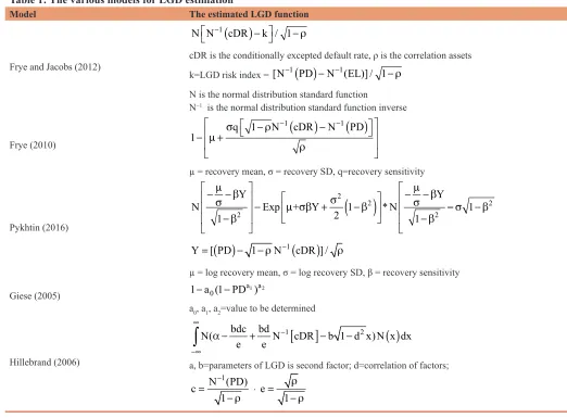
Table 1: The various models for LGD estimation
Model The estimated LGD function
Frye and Jacobs (2012)
N N −1
(
cDR)
−k −/ 1 ρcDR is the conditionally excepted default rate, ρ is the correlation assets k=LGD risk index = [N−1
( )
PD −N−1(EL)] / 1−ρN is the normal distribution standard function
N−1 is the normal distribution standard function inverse
Frye (2010) 1
1 1 1
− + −
(
)
−( )
− −
µ σ ρ ρ
q N cDR N PD
µ = recovery mean, σ = recovery SD, q=recovery sensitivity
Pykhtin (2016)
N
Y
Exp + Y
2 N
Y
2
− − −
− +
( )
−
− − − µ
σ β
β µ σβ
σ β σµ β β
1
1
1
2
2
2
* −− −
σ 1 β2
( )
1(
)
Y [ PD= − 1− ρ N cDR ] /− ρ
µ = log recovery mean, σ = log recovery SD, β = recovery sensitivity
Giese (2005) 1−a0 1−PD )
a1 a2
(
a0, a1, a2=value to be determined
Hillebrand (2006)
[
]
( )
1 2
bdc bd
N( N cDR b 1 d x) N x dx
e e
∞
−
−∞
α − + − −
∫
a, b=parameters of LGD is second factor; d=correlation of factors;
1
N (PD) c
1 −
=
− ρ . e 1
ρ =
The formula for calculating RWA is in the form of:
RWA = K*EAD (1)
EAD1: Is seen as an estimation of the extent to which a bank may
be exposed to counterparty in the event of, and at the time of, that counterparty’s default. EAD is equal to the current amount outstanding in case of fixed exposures like term loans. In our calculation the value of LGD was set at 45%.
K: Is the capital requirement is in the form of:
K
LGD* * PD *
=
−
(
)
( )
+
(
)
−
−
ϕ 1 ϕ ϕ
1
0 999 0 5
1
0 5 1
ρ
ρ 1− ρ
,
, ,
− PPD*LGD *
12 5,
(2)
PD is the probability that the borrower falls default;
LGD is the loss rate in the presence of a default The PDi corresponds to :
PDi = P[Ai<D] With :
PDi is the probability that the borrower i falls default Ai is the asset value i:
D is the value of obligations i:
φ is the normal distribution standard function;
φ−1 is the normal distribution standard function inverse. The PD corresponds to:
PDi = P[Ai<Bi] (3)
With:
Ai is the asset value i
Bi is the value of obligations i
N is the cumulative normal distribution function
N−1 is the cumulative normal distribution function inverse.
3. MODEL SPECIFICATION
3.1. Estimating the Expected LGD
Merton (1974) and Black and Scholes (1973) proposed a simple model of the firm that provides a way of relating credit risk to the capital structure of the firm. In this model the value of the firm’s
assets is assumed to follow a lognormal diffusion process with a constant volatility (Chart 1).
Ai t Ai e
i i t i Xt
, ,
. .
= −
+
0 2
2 µ σ σ
(4)
1 Draft Supervisory Guidance on Internal Ratings-Based Systems for
Corporate Credit.
Xt ~N
( )
0, t(5)
Xt un processus de Wiener avec une attente de 0 et de variance t.
µi represents the expected rate of return on assets σi is the volatility of the return on assets.
ln(Ai t,)=ln A( i, )+ i− i .t i X. t
+
0
2
2
µ σ σ
(6)
=> + −
ln A( i t, ) ~N ln A( i,0) i i . ,t i t 2
2
µ σ σ
(7) So Ai,t follows a lognormal distribution with parameters
ln A( i,0) i i 2
2
+ −
µ σ t and σi t with a density function
g x
x b e
x a b
( )
= −( )−
1 1 2
1 2
2
π
ln
a=ln Ai + i− i t et b i t
=
( ,0) . 2
2
µ σ σ
It is possible to calculate expectancy of Ai,t according to the log normal distribution.
µA i t µ σ σ ln A i i t i t
i t
i E A e ,
, ,
( ) . .
=
( )
= + −
+
0 2
2
2 2
(8)
i,t
i.t A A .ei,0 µ
µ =
(9) 3.2. Conditional Minimum Value
Ammari and Lakhnati (2016) has introduced the notion of the
minimum value of an asset to estimates the LGD:
For a fixed probability α, Minα is defined by
P(Ai,t < Minα) = α (10)
Now we introduce a new notion CMinA
i,α which be called
conditional minimum value:
E(Ai t|Ai t MinA CMinA
i T i
, , < , ,α)= ,α
(11) Which simply represents the minimum conditional value that an
asset may have during a period, with a risk α In the case of Merton model we have:
E(A |A Min
A g A dA P A
i t i t A
Min
i t i t i t i t i T Ai T , , , , , , , , ,, ) / <
=
∫
( )
<α
α
0
M Min
Ai T, ,α
(
)
(12)
=
∫
⋅ −( )
−
1 1 1
2 0 1 2 2 α π α Min i t i t A a b i t
Ai T i t
A
A b e dA
, , ,
, ,
(ln ) , (13) =
∫
−( )
− 1 1 2 0 1 2 2 α π αMin A a
b
i t
Ai T i t
b e dA
, , ,
(ln ) , (14) =
∫
− − 1 2 1 2 2 α −∞ α π ln MinA A a
b
i t Ai T
i t i t e
b e dA
( ) ( ) , , , , , (15) =
∫
− − 1 2 1 2 2α −∞ π
α
ln Min A A a b
i t Ai T i t
i t e b dA ( ) ( ) , , , , , (16) We have A A a b b
A aA a 2b A
(i,t)
i,t
i,t i,t i,t
− − = − − + − = − 1 2 1 2 2 1 2 2 2
2 2 2
( )
b b
(A A a+b ) a
b (A a+b) b a a+ i,t i,t 2 i,t 2 2 2 2 2 2 2 2 2 1 2 1 2 − + = − − + − − ( )
( ) ( ( bb
b
(A a+b) a b
2 i,t ) ) ( ) 2 2 2 2 2 1 2 2 = − − + + (17)
E(A |A Min e
b dA
i t i t A
b A a b a b i i T i t , , , ( ( )) , , ) < = − − + + + α α π 1 2 1
22 2
2 2 2
,, ( ) ( ) ( , , , , , t ln Min
a b ln Min A a b
Ai T
Ai T i t
e e −∞ −∞ α α α
∫
∫
=+ 2 − − + 2 2 1 2
(( )
b i t b dA ) , 2 2π (18)We set s =
A a b
b ds = dA b i t i t ( , ) , − +
(
)
⇒ 2 SoE(A |Ai t i t MinA e e ds
a b ln Min s
i T Ai T , , , ( ( ) , , , ) < = + − − −
α α ∞ π
α 2 2 2 1 2 2 (( ) , ) ( ( ) ( ) ) , a b b a b A =e
ln Min a b
b i T + +
∫
− + 2 2 2 2 α ϕ α (19)φ is the normal distribution standard function;
Ammari and Lakhnati (2016) prouved that MinA a b
i T,,
( ) α= + ϕ α−1
With φ−1 is the normal distribution standard function inverse. So
E(A |A Min e
a b a b
b
i t i t A
a b i T , , , , ) ( ( ) )
< = + − +
(
)
+ −
α α ϕ
ϕ α
2
2 1 2
From E(Ai t|Ai t MinA e b
a b
i T
, , < , , )=
(
( )
−)
+
− α α ϕ ϕ α
2
2
1 (20)
We have a=ln Ai,0 + i- i t and b i t
=
( ) µ . σ
2
2
We deduce that
E(A |Ai t i t MinA e i t ln A i t
i T i , , , ( ) . , , )
< = +
(
−( )
−)
α
µ
α ϕ ϕ α σ
0
1
(21) at t = T=1
( )
(
)
i,0 i,T
ln(A ) i. 1 A , e
CMin +µ − i
α = α ϕ ϕ α − σ (22)
The formula (22) is very useful for financial calculations under the
conditionnel minimum value that could reach the asset Ai at any time
t, specifically at the maturity T, which can be regarded as an expected conditionnal value according to a previously specified risk level.
3.3. Estimated Loss Rate (LGD)
LGD is calculated in various ways, but the most popular is Gross LGD, where total losses are divided by EAD. An alternate method is to divide losses by the unsecured portion of a credit line (where security covers a portion of EAD. This is known as Blanco LGD. If the collateral value is zero in the last case then Blanco LGD is equivalent to gross LGD. A variety of statistical methods may be applied. In this article, the rate of LGD will be calculated according to the minimum value.
With the formula (22), we can already get an idea of the impairment
of financial assets over time (t), which is essential to calculate the rate of percentage loss of the initial value of a financial asset.
In this section, a development of the formula (22) will be established by calculating loss rates (LGD) that could represent
The Chart 2 revealed two losses of asset Ai,t, an average loss and
other unexpected with a level of risk α.
With α lower level of risk, it is possible to calculate an unexpected
loss as in the previous section. This loss will be used to determine
the unexpected loss rate with the use of the initial value of the
asset A as:
Estimation de la LGD:
i,T i,t
i,0 A ,
A ,
i,0
A CMin
LGD
A
α α
− =
(23)
( )
(
)
i,0
i,t
ln(A ) i 1 i,0
A ,
i,0
e
A i
LGD
A
+ µ −
α
− ϕ ϕ α − σ
α
=
(24)
( )
(
)
i,t
i 1 A ,
e i
LGD 1
µ −
α
ϕ ϕ α − σ = −
α (25)
3.3.1. Case of a single asset Ai
When t = T
( )
(
)
i 1
e i
LGD 1
µ −
α
ϕ ϕ α − σ = −
α (26)
α is the risk taken on assets.
3.3.2. Case of two assets
(
)
( )
(
)
i,0 j,0 i j i,t j,t
ln A A (w . i w . j) 1 A A , e
CMin + + µ + µ − ij
+ α = α ϕ ϕ α − σ
(27) wi, wj are weights of the assets i, j
2 2 2 2
i i j j
ij w . i 2* .w .w i. j w j
σ = σ + ρ σ σ + σ
ρ is the correlation between Ai,t and Aj,t
( )
(
)
i j
i j
w . i w . j 1
A A ,
e ij
LGD 1
µ + µ −
+ α
ϕ ϕ α − σ = −
α (28)
3.3.3. Case of several credit portfolio as well
( )
(
)
p i i 1 p
i i 1
w . i 1
A ,
e R
LGD 1 =
=
µ −
α
ϕ ϕ α − = −
α
∑
∑
(29) Such as R = tw∑w
∑ is the variance covariance matrix of the assets
w is the weights matrix of the assets
tw is the transposed weights matrix of the assets.
4. EMPIRICAL RESULTS
4.1. Illustration of the Calculation of the Conditional Minimum Value and the LGD
4.1.1. Case of a single asset
With
n 2
i,j i j 1
2 ( )
i
n 1
= µ − µ σ =
−
∑
and ni,j j 1
i n=
µ
µ =
∑
i
i 16.35% and 7.42%
σ = µ =
We would calculate CMin A ,i,Tα with α = 1% as a risk level from
the 5th year, posing A
i,0 = 7.000.000 Dhs (Table 2).
The Chart 3 shows the distribution of asset Ai, with T = 1.800 (for 3 years) according to a number of simulations, the final value of
i,T
A ,1%
CMin = 4.817.437 DH with LGD 1% = 31.18% which is
equivalent to the Ai loss percentage.
4.1.2. LGD of two assets Ai and Aj
The financial data of a portfolio of two companies are shown in
Table 3.
In this case, we have:
Ai,0 = 7.000.000 µi = 7.42% and σi = 16.35% wi = 0.38
Table 2: Financial data of a Moroccan bank
Company Year Tutnover
(MAD) (MAD)Assets return (%)Rate of
C1 1 17,500,000 7,000,000
2 16,250,000 6,500,000 −7 3 20,000,000 8,000,000 23 4 18,750,000 7,500,000 −6 5 22,500,000 9,000,000 20 Average
Aj,0 = 15.000.000 µi = 15.84% and σi = 26.94% wj = 0.62
Case 1: Separated calculation LGD A i,Tand LGD Aj,T
i,T
A , 1%
CMin = 4.817.437 DH
j,T
A , 1%
CMin = 8.293.882 DH
i,T
A , 1 %
LGD = 31.18% LGD A , 1 %j,T = 44.71%
i,T j,T
A ,1 % A , 1%
Min Min+ = 13.111.319 DH
(
i,T j,T i,T j,T)
A et A , 1%
A A
LGD
separated calculation of LGD and LGD =40.40%
Case 2: Calculation of LGD as in a portfolio of credit assets So we use the formula below,
(
)
( )
(
)
i,0 j,0 i j i,t j,t
ln A A (w . i w . j) 1 A A , e
CMin + + µ + µ − ij
+ α = α ϕ ϕ α − σ
wi,wj are weights of the assets i, j
2 2 2 2
i i j j
ij w . i 2* .w .w i. j w j
σ = σ + ρ σ σ + σ
Asset correlation ρ = −59%
So:
σij = 13.72%
AndCMin Ai,T j,T + A , 1%=18.514.342 Dhs,
i,T j,T
A ,1 %
LGD + 22.86%=
With the second case, a great gain was obtained by the application of the notion of correlation, this is also by the reduction of the
estimated loss rate, which is decreased from 44.44% to 22.86%.
The Chart 4 shows the variation in the estimated LGD loss rate due to the correlation between the two assets Ai and Aj.
It should be noted that the link between the correlation between the two assets and the LDG loss rate is perfectly decreasing, a
Table 3: The financial data of a portfolio of two companies
Company Year Turnover (MAD) Assets (MAD) Rate of return (%) Average return (%) Volatility (%) Asset correlation (%)
C1 1 17,500,000 7,000,000 7.42 16.35 −59
2 16,250,000 6,50,0000 −7
3 20,000,000 8,000,000 23
4 18,750,000 7,500,000 −6
5 22,500,000 9,000,000 20
C2 1 22,500,000 9,000,000 15.84 26.94
2 23,750,000 9,500,000 6
3 21,250,000 8,500,000 −11
4 32,500,000 13,000,000 53
5 37,500,000 15,000,000 15
Chart 3: Determination of the minimum value of the asset Chart 4: Estimated loss rate LGD
10% decrease in the correlation implies an average reduction of 6% for the loss rate.
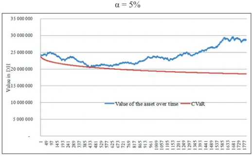
4.2. Back testing of the calculated Conditional Minimum Value
Chart 5 and Table 4 show two simulations of the assets distribution
in two Ai risk levels 1% and 5%, T = 1000.
The objective of this section is to develop a backtesting program for the developed model. It is shown that the greater the number of simulations the greater the importance of estimated power.
For 100 simulations, the exceedance rate is 6.20% for a level of risk of 5%, which is a quality of 76% significance.
For 10.000 simulations, the model becomes more significant with a quality of 99.10%, the exceedance is 5.04% for a risk of 5% and 0.99% for a 1% risk.
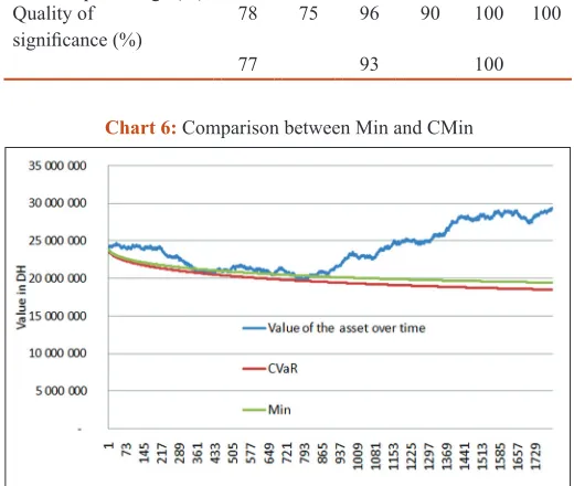
4.3. Comparison Between Min and CMin
We compared the relevance of our model with the model that uses the minimum value to estimate a LGD. The result of this comparison is illustrated in the Chart 6.
By observing the graph above, it should be noted that the
CMin model gives more precision of the potential loss of the asset.
5. CONCLUSIONS
In this article, we estimated the LGD rate, using the Merton
model, by introducing a new parameter that called the conditional minimum value.
Four components were developed in this work: Estimation of the conditional minimum value that an asset could have during a
period, estimation of LGD loss rate, and finally validation of the
proposed model.
We can say that the proposed model makes it possible to calculate the LGD rate in a very simple way, in addition, this model takes
into account the notion of diversification of portfolios, which was
shown by the result section.
It has also been shown that this model gives more accuracy on
the LGD rate than the model based on the Min value. It should be
noted that this is possible to develop a model based on a stressed
minimum value, as a research axis.
Another factor requires a particular analysis, namely the correlation of the assets, this element must be modeled in an adequate way to calculate the weighted assets, in this sense we can cite the work
of AMMARI and Lakhnati (2017).
REFERENCES
Altman, E., Resti, A., Sironi, A. (2004), Default recovery rates in credit risk modeling. A review of the literature and empirical evidence. Economic Notes, 33, 183-208.
Ammari, M., Lakhnati, G. (2016), Loss given default: Estimating by analyzing the distribution of credit assets and validation. Journal of Finance and Investment Analysis, 5, 1-18.
Ammari, M., Lakhnati, G. (2017), Default-implied asset correlation: Empirical study for moroccan companies. International Journal of Economics and Financial Issues, 7(2), 415-425.
Black, F., Scholes, F. (1973), The pricing of options and corporate liabilities. The Journal of Political Economy, 81(3), 637-654. Das, S.R., Hanouna, P. (2006), Credit default swap spreads. Journal of
Investment Management, 4, 93-105.
Frye, J. (2003), A false sense of security. Risk, 16(8), 63-67.
Frye, J. (2010), Modest Means, Risk. Chicago, IL: Federal Reserve Bank. p94-98.
Frye, J., Jacobs, M. (2012), Credit loss and systematic loss given default. Journal of Credit Risk, 8, 1-32.
Giese, G. (2005), The Impact of PD/LGD Correlations on Credit Risk Capital, Risk; 2005. p79-84.
Gupton, G.M. (2005), Advancing loss given default prediction models: How the quiet have quickened. Economic Notes by Banca Dei Paschi di Siena SPA, 34(2), 185-230.
Hillebrand, M. (2006), Modeling and Estimating Dependent Loss Given Default, Risk. Garching, Germany: Munich University of Technology; 2006. p120-125.
Huang, X., Oosterlee, C.W. (2008), Generalized Beta Regression Models for Random Loss-Given-Default. Delft, Delft University of Technology Report 08-10, 2008.
Merton, R. (1974), On the pricing of corporate debt: The risk structure of interest rates. Journal of Finance, 29, 449-470.
Pykhtin, M. (2016), Unexpected recovery risk. Risk, 16(8), 74-78. Schuermann, T. (2004), Easurement, estimation and comparison of
credit migration matrices. Journal of Banking and Finance, 28(11), 2603-2639.
Steinbauer, A., Ivanova, V. (2006), Internal LGD estimation in practice. WILMOTT Magazine, 1, 86-91.
Table 4: Back testing based on number of simulations
Element Number of simulation
100 1000 10,000
Confidence level (%) 5 1 5 1 5 1
Overrun percentage (%) 6.10 1.25 5.20 1.10 5 1 Quality of
significance (%) 78 75 96 90 100 100
77 93 100