Implementation of Graph Theory in Computer Networking To Find an Efficient Routing Algorithm

(1)

ISSN(Online): 2320-9801

ISSN (Print): 2320-9798

I

nternational

J

ournal of

I

nnovative

R

esearch in

C

omputer

and

C

ommunication

E

ngineering

(An ISO 3297: 2007 Certified Organization)

Vol. 4, Issue 1, January 2016

Implementation of Graph Theory in

Computer Networking To Find an Efficient

Routing Algorithm

Mohd Nayeem Shah

I.T Engineer, REEF GLOBAL GROUP, Makkah, Kingdom of Saudi Arabia

Former Assistant Professor (Contractual), Department of Computer Science & Engineering, Islamic University of

Science & Technology, Awantipora, J&k, India

ABSTRACT: In a computer network, the transmission of data is based on the routing protocol which selects the best routes between any two nodes. Different types of routing protocols are applied to specific network environment as one routing protocol which seems to be efficient in one network seems to be inefficient in a different network especially when the number of nodes varies. RIP (Routing Information Protocol) is one of the oldest routing protocols still in service. Hop count is the metric that RIP uses and the hop limit limits the network size that RIP can support. OSPF (Open Shortest Path First) is the most widely used IGP (Interior Gateway Protocol) in large enterprise networks. EIGRP (Enhanced Interior Gateway Routing Protocol) is Cisco's proprietary routing protocol. This paper analyses which computer routing protocol performs the most efficiently. Each protocol is built around a single source shortest path algorithm. MATLAB was used to construct complex scenarios and determine which algorithms are best for graphs of variable lengths.

KEYWORDS: Routing Protocol; graph ; vertices ; shortest path algorithm; BW=BandWidth

I. INTRODUCTION

Networks have been used in a variety of applications for hundreds of years. In the scope of mathematics, we can visually depict these networks better through graphs. A graph is a representation of a group or set of objects, called vertices, in which some of the vertices are connected by links, also known as edges. The study of these graphs is often referred to as Graph Theory. Fig.1 and Fig. 2 are examples of simple graphs.The example used in Fig. 1 is known as an undirected graph, a graph in which the edges have no orientation. A more practical example of an undirected graph would be two people shaking hands. Person A is shaking hands with person Band at the same time, person B is shaking hands with person A.

(2)

ISSN(Online): 2320-9801

ISSN (Print): 2320-9798

I

nternational

J

ournal of

I

nnovative

R

esearch in

C

omputer

and

C

ommunication

E

ngineering

Fig. 2 shows a directed graph, or digraph. A digraph has edges that have direction and are called arcs. Arrows on the arcs are used to show the flow from one node to another. For example, from Fig. 2, vertex 1 can move to vertex 2, but 2 cannot move to 2. Often times, graphs will belabelled with a number on the link. This means that the graph is weighted and this number denotes the cost it takes to get from one vertex to the next.There are many topics being researched today related to Graph Theory. However, the context of this paper will be focused on Shortest Path Algorithms (SPAs). More specifically, we will discuss how SPAs are used in current computer networking technology.A Shortest Path Algorithm is a method that will find the best or least cost path from a given node to another node. Two of the most common SPAs discussed in graph theory today are the Bellman-Ford algorithm and Dijkstra’salgorithm. Computer networking relies deeply on graph theory and shortest path algorithms. Without SPAs, network traffic would have no direction and not know where to go. It is also very important that network traffic does not loop.

An Interior Gateway Protocol is a routing protocol that is used to share routing information within a local Autonomous System (AS). Examples of these routing protocols are Routing Information Protocol (RIP), Open Shortest Path First (OSPF) and Enhanced Interior Gateway Routing Protocol (EIGRP). Each of these algorithms uses a unique method to find shortest paths between network routes. Also, one of the most unique distinctions between each routing protocol is how each chooses their edge weights. RIP considers the cost from vertex to vertex to all be equal. Therefore, the shortest path is determined solely on the shortest number of nodes used to get to the destination. OSPF uses a very simple calculation to find its edge weight. Its cost is found by taking one hundred divided by the bandwidth in units of Megabits per second. EIGRP uses a more complex formula in calculating weight but still does not require much overhead. The cost metric can be found by using the following formula (the K variables are predefined and a default value is most often used).

[{K1×BW+(k2×BW)/(256-Load)+k3×Delay}×k5/(k4+Reliability)] ×256 ,where BW=BandWidth

From the information provided above, it is clear that each algorithm is unique. I studied each of these routing protocols in depth, and analysed the efficiencies of each and worked to find which one is best. It is well known that each of these routing protocols were built around a previously discovered graph theory algorithm. For example, OSPF was created knowing that Dijkstra’s algorithm would be used in finding the shortest path. There have been several revisions of this protocol since its release, but those changes were made to accommodate for new technology.Overall, the method used to find the shortest path has remained the same for years. There are many times where multiple routing protocols find a shortest path to be the same path as another protocol. Therefore, I define efficiency to be equal to the time it takes for an algorithm to actually calculate the shortest path. Given the size of today’s networks, the process of calculating routing paths can be exhausting. Any time a path is modified or changed, the algorithm must be ran again on the network to determine if a new shortest path is available. For example, a cable between two routers being cut would represent an edge being removed from a graph because there is no longer a connection between routers, or vertices. Similarly, when a router is taken out of a network, this represents a vertex being removed from the graph. From past experience in computer networking, the arguments posed on choosing a particular routing protocol are only related to which protocol is best for the type of equipment or connections that are being used. It should also be known that this paper will focus on undirected graphs. In the area of computer networking, it is not practical to say that network traffic can flow in one direction across a given path, but not the other direction. Therefore, directed graphs will be excluded from most of the research topics. I will show my analysis of the shortest path algorithms. Then, I will move in to the experimental portion and explain, in detail, how I used computer software to find the results.

II. RELATED WORK

Shortest Path Algorithms are used in many applications of everyday life. Consider using computer navigation software to obtain directions to a place you have never driven to before. In most cases, there are many paths one could take in order to arrive at that location. This software creates a graph with the vertices representing a physical location and the edges which represent the road that connects two locations. If there is not a road between locations, then there is not an edge in the graph. Next, a weight is associated with each edge. In this example, the primary metric used for weight is distance. However, other factors in this example are considered when assigning a weight, or cost, to an edge, such as traffic and average speed of vehicles on a given road.

(3)

ISSN(Online): 2320-9801

ISSN (Print): 2320-9798

I

nternational

J

ournal of

I

nnovative

R

esearch in

C

omputer

and

C

ommunication

E

ngineering

development began to rise. This time period marked a new era of complex network applications. For example, telephone networks were growing significantly larger, creating a demand for a more efficient process to find the shortest path to the end caller. Before this period, call routing had to be completed manually by telephone operators. Therefore, if a particular call path was broken, it was not automatically intuitive as to which backup path should be taken. While several mathematicians and computer scientists contributed to this research, two major contributions were Edsger Dijkstra and Dijkstra’s algorithm in 1956 and also the Bellman-Ford algorithm, developed by Lester Ford, Jr. and Richard Bellman in 1956 and 1958 respectively. The Bellman-Ford algorithm was also published in 1957 by Edward F. Moore and is sometimes referred to as the Bellman-Ford-Moore algorithm. Computer networks began to evolve throughout the late 1950s and 1960s. The majority of these networks were initially used in military operations for top secret data transfer and also for radar system Semi-Automatic Ground Environment (SAGE) [1] . This created a great opportunity for computer networking in the corporate world as well. American Airlines was the first American company to fully utilize a complex network to connect mainframe systems for the use of Semi-automated Business Research Environment (SABRE).

As corporate networks began to grow, it became very difficult to manually manage every connection between sites. Configuring routers to direct traffic to a fixed location at all times was completely inefficient. Routers needed the ability to dynamically calculate the best and shortest path quickly. This process is referred to as dynamic routing. The first major dynamic routing protocol, Routing Information Protocol (RIP), was implemented in 1988. “This algorithm has been used for routing computations in computer networks since the early days for the ARPANET” (RFC 1058). RIP runs as a software component on routers based on the Bellman-Ford algorithm. Each routing protocol uses a different method in calculating the cost between routers. RIP determines that the hop count is the routing metric. RIP is still commonly used in networks today. The second major dynamic routing protocol is called Open Shortest Path First (OSPF). This protocol is current on version 2, which is defined by RFC 2328 and published by the Internet Engineering Task Force (IETF) in 1998. Similarly, OSPF exercises a previously defined shortest path algorithm, Dijkstra’s Algorithm. OSPF calculates determines the bandwidth between two routers and then assigns that bandwidth amount in megabits per second to the edge cost. This protocol is also implemented frequently in corporate networks around the world today.

III.SHORTEST PATH ALGORITHMS

Now I will define each shortest path algorithm. Take a weighted digraph G = (V, E). I denote the letter G as the name of the graph, V to be a representation of all the vertices in the graph, and E to contain all the edges between vertices. Given a source and destination vertex, it can be said that a sequential list of vertices which connect the source and destination can be called a path, where

= 1 → 2 → ⋯→ .

The edge weights can be given by a function

∶ → R.

Therefore, the weight can be written as follows: ( ) = ∑ (vi, vi+1)

After taking the sum of edges used for each path, the path that has the smallest sum can be known as the shortest path. We can now define the shortest path weight to be

( , ) = min{ ( ): ℎ }.

(4)

ISSN(Online): 2320-9801

ISSN (Print): 2320-9798

I

nternational

J

ournal of

I

nnovative

R

esearch in

C

omputer

and

C

ommunication

E

ngineering

From Fig. 3 illustrates two possible paths from vertex A to D. Those paths are A-C-D and A-B-C-D. The Brute-Force algorithm will first find all paths without considering the edge weights. Once all paths are found, the algorithm will then find the shortest path. In simple networks, there is not usually a problem with using the Brute-Force method. However, as the graph grows larger, the Brute-Force requires many more computations. Now, it will be helpful to look at the Single-Source Shortest Path algorithms[7]. These are algorithms that from any given source vertex ∈ they will find the shortest path ( , ), ∀ ∈ . To date, there is not an efficient algorithm that can find the shortest path from one vertex to another specific vertex without taking into consideration the other vertices in the graph[3]. After the distance from the source to the other vertices has been calculated, it will be easy to back track to find the path. Dijkstra’s Algorithm is the most common single-source shortest path algorithm. It will require three inputs (G, w, s), the graph G (containing vertices and edges, the weights w, and the source vertex s. Dijkstra’s Algorithm is outlined as follows:

( , , ) [ ] = 0

ℎ ∈ − { } [ ] = ∞

= ∅

=

ℎ ≠ ∅

= ( ) = ∪ { }

ℎ ∈ { } [ ] > [ ] + ( , )

ℎ [ ] = [ ] + ( , )

Dijkstra’s algorithm must first initialize its three important arrays. First, the array S contains the vertices that have already been examined or relaxed. It first starts as the empty set, but as the algorithm progresses, it will fill it with each vertex until all are examined. Then, the distance array d[x] is defined to be an array of the shortest paths from s to x, or also denoted ( , ) ℎ ∈ . Finally, Q is simply the data type used to form the list of vertices. In this case, we call it a priority queue. Even though Dijkstra’s algorithm appears to be very efficient, it must only consider non negative cost values on the edges, as having a negative value can result in an unwanted loop. However, this is not an immediate concern from our study, because in each of our networking protocols, there cannot be a negative metric value.

(5)

ISSN(Online): 2320-9801

ISSN (Print): 2320-9798

I

nternational

J

ournal of

I

nnovative

R

esearch in

C

omputer

and

C

ommunication

E

ngineering

Now I will analyse Bellman-Ford algorithm, which can be seen below. ( , , )

[ ] = 0

ℎ ∈ − { } [ ] = ∞

= 1 | | − 1 ℎ ( , ) ∈

[ ] > [ ] + ( , )

ℎ [ ] = [ ] + ( , )

The Bellman-Ford algorithm takes the same approach for initialization as Dijkstra. It will also accept the graph to be input as a square matrix. Bellman-Ford is known to be fairly simple but not run as efficiently. This shortest path algorithm will be controlled by a “for-loop” that runs |V| - 1 iterations where |V| is equal to the number of vertices in the network. Bellman-Ford will now run the same relaxation test as Dijkstra for each edge in the graph. Upon completion of each relaxation, the shortest path will be found [6]. I can now move to the experimental test where I can code these algorithms and test their results.

IV.SIMULATION RESULTS

Before jumping into the analysis of these algorithms, it is important for me to choose a mathematics software that best fit. I used MATLAB because it is matrix-oriented and seemed to be the most efficient for making fast calculations. In order to input data into the MATLAB functions, I had to have some sort of method in which to describe the graphs. I choseto input the graph in the form of a square matrix. The matrix will always be of n x n dimension where n is equal to the number of vertices in the graph. Each row will represent the vertex from which we are traveling. Each column will represent the vertex to which we are traveling to [2]. The matrix G is a representation of the graph with three vertices. Vertex A corresponds to row and column 1, B to row and column 2, etc. Matrix G shown is the matrix representation of the graphgraph in Fig. 4.

(6)

ISSN(Online): 2320-9801

ISSN (Print): 2320-9798

I

nternational

J

ournal of

I

nnovative

R

esearch in

C

omputer

and

C

ommunication

E

ngineering

call. The next large task faced was creating random graphs. I created a function named buildMatrix() to build our graph. This function runs in ( 2) time, where n equals the number of nodes.

Initially, the function creates n by n matrix with random numbers between 0 and 1 as elements. Obviously, we do not want a completely random matrix. As previously discussed, we need to have the elements on the diagonal of the matrix equal to zero. Also, the elements need to follow the symmetric property previous discussed, ( , ) = ( , ). Therefore, the “If-Then” command controlled by the nested loop analyses if the element is on the diagonal. If it is, then the function sets that value equal to zero. If the element is not on the diagonal, it will set the corresponding element on the other side of the diagonal such that ( , ) = ( , ). It was not practical to have each element in the graph, excluding the diagonal, set to a value greater than zero. If each value was greater than zero, this would imply that the graph is complete, or fully meshed. “A complete graph is a simple undirected graph in which every pair of distinct vertices is connected by a unique edge. Fig. 5 is an example of a complete graph with six vertices.

(7)

ISSN(Online): 2320-9801

ISSN (Print): 2320-9798

I

nternational

J

ournal of

I

nnovative

R

esearch in

C

omputer

and

C

ommunication

E

ngineering

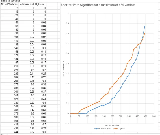
The “tic-toc” pre-defined MATLAB function is used each time to determine the time taken for each algorithm to run. The time recordings are stored in to a variable called Results. After the driver.m program has completed, we imported these values into a Microsoft Excel spreadsheet in order to easily create graphs and mine the data easily.

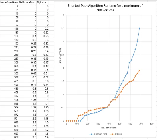
Fig. 6&Fig. 7 are line graphs from runtimes of both major SPA’s. Fig. 6 exhibits 1 to 450 vertices while Fig. 7 shows runtimes for 1 to 700 vertices. After running the two single-source shortest path algorithms, it can be seen that the Bellman-Ford algorithm is more efficient than Dijkstra’s algorithm until the number of vertices in the graph reach around 425. From this point, Dijkstra’s algorithm shows to be much more efficient as the number of vertices approach infinity.

Time in seconds

No. of Vertices Bellman-Ford Dijkstra

2 0 0

15 0 0

28 0 0

41 0 0

54 0 0.02

67 0 0.04

80 0 0.05

93 0 0.06

106 0.02 0.07

119 0.03 0.08

132 0.04 0.09

145 0.05 0.1

158 0.06 0.11

171 0.07 0.12

184 0.08 0.15

197 0.08 0.17

210 0.09 0.19

223 0.1 0.2

236 0.11 0.25

249 0.15 0.27

262 0.16 0.3

275 0.2 0.32

288 0.22 0.35

301 0.26 0.37

314 0.3 0.4

327 0.33 0.44

340 0.37 0.5

353 0.4 0.53

366 0.47 0.56

379 0.5 0.64

392 0.54 0.66

405 0.6 0.69

418 0.7 0.7

431 0.76 0.74

444 0.87 0.8

-0.1 0 0.1 0.2 0.3 0.4 0.5 0.6 0.7 0.8 0.9 1

0 50 100 150 200 250 300 350 400 450 500

Ti m e in s ec o n d s

No. of vertices

Shortest Path Algorithm for a maximum of 450 vertices

Bellman-Ford Dijkstra

(8)

ISSN(Online): 2320-9801

ISSN (Print): 2320-9798

I

nternational

J

ournal of

I

nnovative

R

esearch in

C

omputer

and

C

ommunication

E

ngineering

Time in seconds

No. of vertices Bellman-Ford Dijkstra

2 0 0

21 0 0

40 0 0

59 0 0

78 0 0

97 0 0

116 0 0.2

135 0 0.22

154 0.1 0.23

173 0.2 0.3

192 0.22 0.32

211 0.24 0.38

230 0.28 0.4

268 0.3 0.43

287 0.33 0.45

306 0.35 0.47

325 0.4 0.49

344 0.46 0.5

363 0.49 0.51

382 0.5 0.52

401 0.6 0.6

420 0.74 0.74

439 0.8 0.8

458 0.9 0.8

477 1.1 0.9

496 1.25 1

515 1.4 1.1

534 1.52 1.25

553 1.7 1.35

572 1.8 1.4

591 2.2 1.48

610 2.3 1.5

629 2.5 1.55

648 2.7 1.7

667 3 1.8

686 3.5 1.9

0 0.5 1 1.5 2 2.5 3 3.5 4

0 100 200 300 400 500 600 700 800

Ti

m

e

in

s

ec

o

n

d

s

No. of vertices

Shortest Path Algorithm Runtime for a maximum of

700 vertices

Bellman-Ford Dijkstra

(9)

ISSN(Online): 2320-9801

ISSN (Print): 2320-9798

I

nternational

J

ournal of

I

nnovative

R

esearch in

C

omputer

and

C

ommunication

E

ngineering

V. CONCLUSION

From the information provided in our Experimental data, it is obvious to see that the brute-force algorithm is not efficient. However, this was expected because every possible path was found without taking the cost into consideration. For very small networks, the brute-force algorithm might be a valid method. It is certainly the easiest for elementary graph theorist to comprehend, but it is not realistic to use this algorithm for very large numbers of vertices. The Bellman-Ford algorithm and Dijkstra’s algorithm proved to be much more efficient than brute-force, with Dijkstra proving to run in the least amount of time for very large networks. It appears that for complete, fully meshed networks, the Bellman-Ford algorithm actually ran faster than Dijkstra’s algorithm for networks of size 425 or less. However, Dijkstra showed to be considerably more efficient beyond networks with more than 425 vertices. As a general rule, network engineers are told to stay away from the routing protocols that use the Bellman-Ford algorithm. Again, these protocols are RIP and EIGRP, while OSPF runs Dijkstra’s algorithm. However, this studies show that for small and medium sized networks, EIGRP and OSPF calculate the shortest path in a relatively close amount of time. Therefore, it can be said that OSPF only needs to be chosen in very large networks. Otherwise, in most cases, EIGRP and OSPF are very similar in their efficiencies.

REFERENCES

1. Schrijver, Alexander. 2010. On the History of the Shortest Path Problem. Documenta Math. p. 155-165. 2. Yellen, Jay and Gross, Jonathan. 2008. Graph Theory and its Applications. Chapman & Hall. P. 172. 3. McHugh, James. Algorithmic Graph Theory. Prentice Hall. P. 92.

4. “Introduction to Algorithms – Lecture 18”. MIT 6.046J. http://www.youtube.com/watch?v=Ttezuzs39nk

5. Wu, Bang Ye. Study of Shortest Path. Shortest-Path Trees.

6. R. Bellman. On a routing problem. Quar. Appl. Math., 16:87-90, 1958.

7. E.W. Dijkstra. A note on two problems in connection with graphs. Numer. Math., 1:269–271, 1959.

BIOGRAPHY