Mixed FEM-BEM Formulations Applied to
Soil-Structure Interaction Problems
Dimas Betioli Ribeiro and Jo˜ao Batista de Paiva
Abstract—The objective of this paper is to present formula-tions developed for soil-building interaction analysis, including foundations. The soil is modeled with the boundary element method (BEM) as a layered solid which may be finite for the vertical direction, but is always infinite for radial directions. Beams, collums and piles are modeled with the finite element method (FEM) using one dimensional elements. Slabs and rafts are also modeled with the FEM, but with two dimensional elements. The analysis is static and all materials are considered homogeneous, isotropic, elastic and with linear behavior.
Index Terms—boundary elements, finite elements, soil-structure interaction.
I. INTRODUCTION
The construction of buildings involve complex soil-structure interaction effects that require previous studies to be correctly considered in the project. The basis of these studies has to be chosen among many options available and each one of them implies on advantages and disadvantages, as described below.
When possible, a good choice is to employ analytical methods. When correctly programmed they give trustful results in little processing time. In reference [1], for example, a solution is presented for an axially loaded pile with a rectangular cross section and immersed in a layered isotropic domain. The main disadvantage of these solutions is that they suit only specific situations, so many researches keep developing new ones to include new problems. Other works that may be cited are [2], [3].
If analytical solutions cannot be used, one alternative could be a numerical approach. The developments [4] of the numerical methods in the latter years and its versatility made them attractive to many researchers. The finite element method (FEM) is still popular [5], [6], [7], [8], however has some disadvantages when compared to other options such as the boundary element method (BEM). The FEM require the discretization of the domain, which has to be simulated as infinite in most soil-structure interaction problems. This implies on a high number of elements, leading to a large and sometimes impracticable processing time.
It becomes more viable solving these problems with the BEM, once only the boundary of the domains involved is discretized. This allows reducing the problem dimension, implying on less processing time. This advantage is explored in several works [9], [10], [11], [12], [13], [14], [15], [16] and new developments are making the BEM even more attractive
Manuscript received March 21, 2014; revised March 25, 2014. This work was supported by the research council FAPESP.
D. B. Ribeiro is with the Department of Structural and Geotechnical Engineering, Polytechnic School of the University of S˜ao Paulo, S˜ao Paulo, SP, 05508-070 Brazil e-mail: [email protected].
[image:1.595.354.497.163.279.2]J. B. Paiva is with the School of Engineering of S˜ao Carlos, University of S˜ao Paulo, S˜ao Carlos, SP, 13566-590 Brazil e-mail: [email protected].
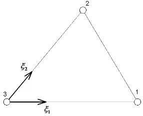
Fig. 1. Triangular boundary element.
to future applications. One is simulating non-homogeneous domains using an alternative multi-domain BEM technique [17], another is using mapping functions to make boundary elements infinite [18].
The objective of this paper is to present a formulation for building-soil interaction analysis that uses recent devel-opments accomplished by the authors in references [17], [18]. The proposed formulation is applied into two examples to show all functionalities of the proposed formulation, considering a piled raft and a complete building interacting with a layered soil. The results obtained may be considered coherent. Finally, it is concluded that the presented formula-tion may be considered a practical and attractive alternative in the field of soil-structure interaction simulation.
II. BOUNDARY ELEMENT FORMULATION The equilibrium of a solid body can be represented by a boundary integral equation called the Somigliana Identity, which for homogeneous, isotropic and linear-elastic domains is
cij(y)uj(y) +R
Γ p∗
ij(x, y)uj(x)dΓ (x) =R
Γ u∗
ij(x, y)pj(x)dΓ (x) (1)
Equation (1) is written for a source pointyat the boundary, where the displacement is uj(y). The constant cij depends
on the Poisson ratio and the boundary geometry at y, as pointed out in reference [20]. The field point x goes through the whole boundary Γ, where displacements are uj(x)and tractions arepj(x). The integral kernelsu∗ij(x, y)
andp∗
ij(x, y)are Kelvin three-dimensional fundamental
so-lutions for displacements and tractions, respectively. Kernel u∗
ij(x, y)has order1/rand kernelp∗ij(x, y)order1
r2, where r=|x−y|, so the integrals have singularity problems when xapproachesy. Therefore the stronger singular integral, over the traction kernel, has to be defined in terms of a Cauchy Principal Value (CPV).
approximated by known shape functions. Here these regions are of two types, finite boundary elements (BEs) and infinite boundary elements (IBEs). The BEs employed are triangular, as shown in Figure 1 with the local system of coordinates, ξ1ξ2, and the local node numbering. The following approx-imations are used for this BE:
uj =
3 X
k=1
Nkukj, pj =
3 X
k=1
Nkpkj (2)
Equation (2) relates the boundary values uj and pj to
the nodal values of the BE. The BEs have 3 nodes and for each node there are three components of displacement uk
j and tractionpkj. The shape functionsNk used for these
approximations are
N1=ξ1, N2=ξ2, N3= 1−ξ1−ξ2 (3) The same shape functions are used to approximate the boundary geometry:
xj=
3 X
k=1
Nkxkj (4)
wherexk
j are the node coordinates. The same functions are
also used to interpolate displacements and tractions for the IBEs:
uj = N p
X
k=1
Nkukj, pj = N p
X
k=1
Nkpkj (5)
Each IBE hasN pnodes and not the3that the BEs have. The IBE geometry, on the other hand, is approximated by special mapping functions.
By substituting Equations (2) and (5) in (1), Equation (6) is obtained:
cijuj+ NBE P e=1 3 P k=1
∆pek ijukj
+ NI BE
P e=1 N p P k=1 ∆∞ pek ijukj
=N BE P e=1 3 P k=1
∆uek ijpkj
+N I BE P e=1 N p P k=1 ∆∞ uek ijpkj
(6) NBE is the number of BEs andNIBE is the number of IBEs.
For BEs:
∆pekij =
Z
γe
|J|Nkp∗
ij(x, y)dγe (7)
∆uekij =
Z
γe
|J|Nku∗
ij(x, y)dγe (8)
In Equations (7) and (8), γe represents the domain of
element e in the local coordinate system and the global system of coordinates is transformed to the local one by the Jacobian |J|= 2A, whereA is the element area in the global system. On the other hand, for IBEs:
∆∞
pekij =
Z
γe |∞
J|Nkp∗
ij(x, y)dγe (9)
∆∞
uekij =
Z
γe |∞
J|Nku∗
ij(x, y)dγe (10)
[image:2.595.306.557.56.167.2]Equations (9) and (10) are analogous to (7) and (8). Integrals of Equations (7), (8), (9) and (10) are calculated by standard BEM techniques. Non-singular integrals are evalu-ated numerically by using integration points. The singular
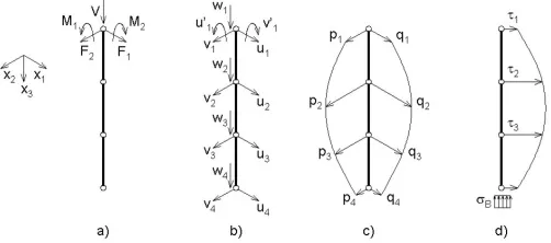
Fig. 2. Model for load lines.
ones, on the other hand, are evaluated by the technique presented in reference [19]. Finally, the free term cij may
be obtained by rigid body motions. Writing Equation (6) for all boundary nodes leads to the following system:
∆p·u= ∆u·p (11)
The∆pek ij and∆
∞
pek
ij element contributions, including the
free termcij, are assembled into matrix∆p, while∆uekij and ∆∞
uek
ij contributions are assembled into matrix∆u. Vectors
u and p contain all boundary displacements and tractions, respectively. Reorganizing this system so as to separate the known boundary values from the unknown yields a system of equations whose solution is all the unknown boundary values.
III. LOAD LINES IN THE SOIL
In this work, the reactive tractions from the piles are applied in the soil as load lines. Figure 2 presents the model adopted, with four nodes equally spaced along the pile.
The load lines influence may be computed in Equation (1) with an additional term as follows
cijuj+
Z
Γ p∗
ijujdΓ =
Z
Γ u∗
ijpjdΓ + nl X e=1 Z Γe u∗
ijsejdΓe
(12) wherenl is the number of load lines, Γe are their external
surface and se
j are the tractions presented in Figures 2c
and 2d. The tractions are approximated from the nodal values sek
j using nf polynomial shape functionsφ:
se j=
nf
X
k=1 φksek
j (13)
Shape functions are written with a dimensionless coordi-nate ξ = 2x3/L−1, where L is the load line length and x3 is the vertical global coordinate. One may observe that −1 ≤ ξ≤ 1, so the use of Gauss points is facilitated. For the horizontal tractions, illustrated in Figure 2c,nf = 4and the shape functions are:
φ1= 1 16 −9ξ
3+ 9
ξ2+ξ−1
(14)
φ2= 1 16 27ξ
3
−9ξ2−27ξ+ 9
(15)
φ3= 1 16 −27ξ
3−9
ξ2+ 27ξ+ 9
(16)
φ4= 1 16 9ξ
3
+ 9ξ2−ξ−1
For shear tractions in direction x3,nf = 3 and the shape functions are
φ1=1 8 9ξ
2−1
(18)
φ2=1
4 −9ξ
2−6ξ+ 3
(19)
φ3=1 8 9ξ
2+ 12 ξ+ 3
(20)
Finally, for the base reaction nf = 1 and a constant approximation is used. Using the shape functions presented above, the integrals that are not singular may be numerically calculated using Gauss points. The term referent to the load lines becomes singular only when the source point belongs to a load line base which is being integrated. In this case, the integral calculation is analytical.
Writing Equation (12) for all boundary points plus the points defined on each load line, the following system of equations is obtained:
[H]{u}= [G]{p} −[M]{s} (21)
Matrix[M]is obtained from the integrals calculated for all load lines, and vector {s} contains the tractions prescribed for them. As the number of equations is equal to the number of unknowns, the system may be solved obtaining all unknowns.
IV. FEM-BEM COUPLING
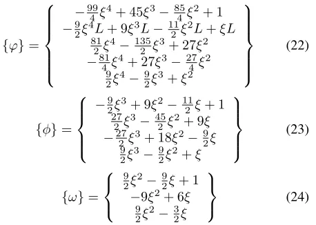
Each pile is modeled using a single finite element with polynomial shape functions. Lateral displacements are ap-proximated using fourth degree polynomials {ϕ}. Vertical displacements and lateral tractions are approximated using third degree polynomials {φ}. Vertical tractions are ap-proximated using second degree polynomials {ω} and the tractions at the pile base are considered constant. Using a dimensionless coordinate ξ = x3
L, where x3 is the global
vertical coordinate and L is the pile length,{ϕ}, {φ} and {ω}may be written as:
{ϕ}= −99 4ξ
4+ 45ξ3−85 4ξ
2+ 1 −9
2ξ
4L+ 9ξ3L−11 2ξ
2L+ξL 81
2ξ 4−135
2 ξ
3+ 27ξ2 −81
4ξ
4+ 27ξ3−27 4ξ
2 9
2ξ 4−9
2ξ 3+ξ2
(22) {φ}= −9 2ξ
3+ 9ξ2−11 2ξ+ 1 27
2ξ 3−45
2ξ 2+ 9ξ −27
2ξ
3+ 18ξ2−9 2ξ 9
2ξ 3−9
2ξ 2+ξ
(23) {ω}= 9 2ξ
2−9 2ξ+ 1 −9ξ2+ 6ξ
9 2ξ
2−3 2ξ
(24)
The next step is obtaining the total potential energy function, considering internal and external contributions. To obtain the final system of equations, such function must be minimized with respect to the nodal parameters. The result is:
[K]{u}={f} −[Q]{y} →[K]{u}={f} − {r} (25)
[image:3.595.68.297.512.675.2]where [K] is the stiffness matrix of the pile, {u} contains nodal displacements,{f}contains nodal loads,{y}contains
Fig. 3. Triangular finite element.
distributed tractions and [Q] is a matrix that transforms distributed tractions into nodal loads. Therefore,{r}contains nodal loads that represent the distributed loads.
Now a brief description of the triangular finite element used for the raft and slabs will be presented. The element has three nodes at its vertices as presented in Figure 3a with the local node numbering and a local rectangular system of coordinatesxi, where the superscriptiindicates the direction.
Each node, indicated with the subscript j, has six degrees of freedom (DOFs). Three of them, uj, vj and θ3j, may
be visualized in Figure 3b which refers to the membrane effects. The other three, wj, θ1j and θ2j, are presented in
Figure 3c which refers to the plate effects. In Figure 3c, rotational DOFs are indicated with a double arrow for better visualization. All DOFs of the finite element may be arranged into three vectors, one for each node, as shown below:
{u1}T = u1 v1 θ13 w1 θ11 θ12
{u2}T = u2 v2 θ23 w2 θ21 θ22
{u3}T = u3 v3 θ33 w3 θ31 θ32
(26)
Displacements at any pointP of the finite element, with coordinatesx1,x2 andx3, may be written as
{u}=
u v w =
u0−x3∂w0
∂x1
v0−x3∂w0
∂x2 w0 (27)
whereu0,v0, andw0are the displacements for the projection ofP at the mid plane of the finite element. The strain field may be obtained from the displacements as follows:
{ε}={εm}+{εp}=
∂u0 ∂x1 ∂v0 ∂x2 ∂u0
∂x2 +
∂v0 ∂x1 −x3 ∂2 w0
∂x12
∂2
w0
∂x22
2 ∂2
w0
∂x1∂x2
(28) where indexmcorresponds to the membrane effect and the index pindicates the plate effect. Equation (28) relates the strain field to the displacement field, which may be related to the nodal displacements using the element shape functions. Using these functions and Equation (28), it is possible to relate strains with the DOFs of the finite element as follows:
{ε}= [B]
u1 u2 u3 (29)
It is also necessary to relate strains with stresses. For linear elasticity this may be done using a matrix [D] which is obtained from Hooke’s law:
In the end, the stiffness matrix of the element is obtained by integrating the domain Ωof the element:
[K] =
Z
Ω
[B]T[D] [B]dΩ (31)
More detail about the membrane and plate effects of this element may be consulted in references [21] and [22], respectively.
All finite element contributions, including piles and the raft, are assembled to the same system of equations. This system has the form of Equation (25), which is later used to demonstrate how the FEM/BEM coupling is made. The starting point is Equation (21), which may be rewritten as:
[H]{u}= [T]{y} (32) Matrix [T] contains the terms of matrices [G] and [M]
and {y} contains the distributed loads of vectors {p} and {s}. Next step is isolating the distributed loads, which are transformed in nodal loads using a matrix[Q].
[T]−1
[H]{u}={y} →[B]{u}={y} (33)
[Q] [B]{u}= [Q]{y} →[D]{u}={r} (34) Before relating Equations (25) and (34), they must be expanded as to contain all degrees of freedom defined in the coupled FEM-BEM model. The result is
¯ K
{u¯F EM}=
¯
f − {r¯F EM} (35)
¯ D
{u¯BEM}={r¯BEM} (36)
These equations are related by imposing compatibility and equilibrium conditions, which are {u¯F EM} = {u¯BEM} =
{u}¯ and {r¯F EM} = {r¯BEM} = {¯r}. The following
expressions are then obtained:
¯ K
{u}¯ =¯ f −¯
D
{u}¯ (37)
¯ K
+¯ D
{u}¯ =¯
f (38)
¯ A
{u}¯ =¯
f (39)
where{¯u} contain all unknown displacements of the FEM-BEM model. Once the number of equations is equal to the number of unknowns, the system may be solved obtaining all unknowns.
V. EXAMPLES A. Piled raft on a layered domain
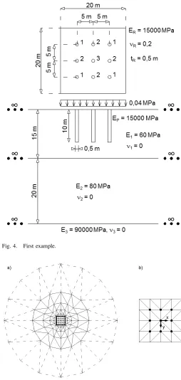
A raft with nine piles on a layered domain is considered, as presented in Figure 4 with all geometrical and material parameters. Young’s module is represented as E, Poisson Ratio as ν and thickness as t. The R subscript indicates the raft, P indicates piles and numbers refer to layers. All piles diameter is 0,5 m and are numbered considering the symmetry planes. The raft is uniformly loaded with 0,04
M P a.
Figure 5a contains the mesh used for the surface and contacts, with160BEs and32IBEs. Figure 5b contains the FE mesh employed for the raft, with the pile positions de-tached. For piles a one-dimensional FE is used, as previously presented.
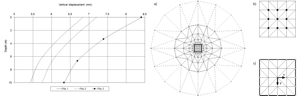
[image:4.595.301.555.58.592.2]Figure 6 presents vertical displacements along the piles, using numbers defined in Figure 4. Pile 3 has the larger
Fig. 4. First example.
Fig. 5. Mesh employed.
displacements, followed by piles 2 and piles 1 with the smaller ones. The result was also symmetric as expected and the magnitude of the values is coherent. This facts allow to conclude the the values here obtained are trustworthy.
B. Building resting on a layered domain
Fig. 6. Displacements for distributed load.
Fig. 7. Soil-building interaction
floor considered and in Figure 7c is presented the top view of the structural foundations included.
The Poisson Ratio is zero for all soil layers. The elasticity modulus of the layers is60M P afor the top one,80M P a for the second and 90000 M P a for the base layer. The thickness is 15 m for the top layer, 20 m for the second and the base layer is considered infinite. The diameter of all piles is0,5m, their length is10mand they are spaced of5
m. The square raft has size20mand thickness0,5m. The elasticity modulus of all materials modeled with the FEM is
15000M P aand their Poisson ratio is0,2. This includes all piles, beams, columns, slabs and the raft.
The building has four floors, as shown in Figure 7a. All floors have the same standard geometry, as presented in Figure 7b, with a slab with thickness 0,3 m, four beams supporting this slab and four columns supporting the beams. A square cross section size 1 m is used for all beams and columns. The base of each column is connected to the raft at the same node where a corner pile is connected. Corner piles are numerated in Figure 7c as 1,3,7and9.
Figure 8 presents the FE-BE-IBE mesh employed in the example. Figure 8a contains the top view of the mesh used for the soil surface and contacts between layers, totalizing
[image:5.595.52.302.246.429.2]480 BEs and 96 IBEs. The square detached at the center indicates the position of the raft at the surface. In Figure 8b is illustrated the mesh with 32 FEs used for the raft,
Fig. 8. FE/BE/IBE mesh employed
together with the position of the piles. Finally, Figure 8c contains the32 FE mesh used for the slabs. Lines detached at the boundary indicate the FEs used for beams, totalizing
16FEs for each floor. Furthermore, each part of the columns between floors is divided into4 FEs. Considering all floors plus the raft, the total number of two-dimensional FEs is160
and the total of one-dimensional FEs is128.
Piles are also simulated with the FEM, employing the FE with14parameters presented previously. The axis of any pile is orthogonal to the surface of the soil.
Fig. 9. Horizontal loads applied
Two horizontal forces are applied at lateral points of the building, as shown in Figure 9. In Figure 9a is presented a lateral view of the structure, with the external forces contained in the plane of the fourth floor. Figure 9b shows a top view, where the position of the forces may be visualized from another perspective.
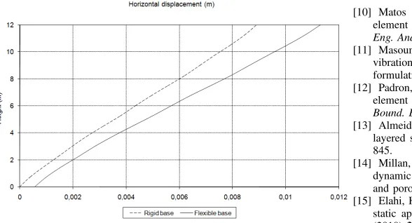
Considering these loads, Figure 10 contains the horizontal displacements calculated for columnC1, which position may be observed in Figure 7b. In this case two simulations were also performed, one considering the flexible base illustrated in Figure 7a and another considering a rigid base. The rigid base was represented restraining displacements at the base node of all columns.
Fig. 10. Horizontal displacement of columnC1
may produce moments that cannot be unvalued and could compromise the safety of the structure. This demonstrates that it is important to include the flexibility of the foundations when projecting buildings.
VI. CONCLUSIONS
In this paper a formulation for building-soil interaction analysis was presented. The FEM/BEM equations together with the techniques from references [17], [18] contributed with reducing the total number of degrees of freedom. Piles are modeled using one-dimensional FEs, whose influence in the soil is computed by integrating load lines. Two examples were presented. In both of them the results obtained were considered coherent. In the end, it may be concluded that the presented formulation is a powerful and attractive alternative for soil-structure interaction analysis.
ACKNOWLEDGEMENTS
Thanks are due to the research council FAPESP and the University of S˜ao Paulo.
REFERENCES
[1] Basu, D., Prezzi, M., Salgado, R. and Chakraborty, T. Settlement analysis of piles with rectangular cross sections in multi-layered soils, Comput. Geotech.(2008)35:563–575.
[2] Shahmohamadi, M., Khojasteh, A., Rahimian, M. and Pak, R.Y.S. Axial soil-pile interaction in a transversely isotropic half-space,Int. J. Eng. Sci.(2011)49:934–949.
[3] Georgiadis, K., Georgiadis, M. and Anagnostopoulos, C. Lateral bearing capacity of rigid piles near clay slopes,Soils. Found.(2013)53:144– 154.
[4] Clouteau, D., Cottereau, R. and Lombaert, G. Dynamics of structures coupled with elastic media - A review of numerical models and methods,J. Sound Vib.(2013)332:2415–2436.
[5] Kim, Y. and Jeong, S. Analysis of soil resistance on laterally loaded piles based on 3D soilpile interaction,Comput. Geotech.(2011)38:248– 257.
[6] Bourgeois, E., de Buhan, P. and Hassen, G. Settlement analysis of piled-raft foundations by means of a multiphase model accounting for soil-pile interactions,Comput. Geotech.(2012)46:26–38.
[7] Su, D. and Li, J.H. Three-dimensional finite element study of a single pile response to multidirectional lateral loadings incorporating the simplified state-dependent dilatancy model,Comput. Geotech. (2013) 50:129–142.
[8] Peng, J.R., Rouainia, M. and Clarke, B.G. Finite element analysis of laterally loaded fin piles,Comput. Struct.(2010)88:1239–1247. [9] Ai, Z.Y. and Cheng, Y.C. Analysis of vertically loaded piles in
multi-layered transversely isotropic soils by BEM,Eng. Anal. Bound. Elem. (2013)37:327–335.
[10] Matos Filho, R., Mendonc¸a, A.V. and Paiva, J.B. Static boundary element analysis of piles submitted to horizontal and vertical loads, Eng. Anal. Bound. Elem.(2005)29:195–203.
[11] Masoumi, H.R., Degrande, G. and Lombaer, G. Prediction of free field vibrations due to pile driving using a dynamic soilstructure interaction formulation,Soil Dyn. Earthq. Eng.(2007)27:126–143.
[12] Padron, L.A., Aznarez, J.J. and Maeso O. 3-D boundary elementfinite element method for the dynamic analysis of piled buildings,Eng. Anal. Bound. Elem.(2011)35:465–477.
[13] Almeida, V.S. and Paiva, J.B. Static analysis of soil/pile interaction in layered soil by BEM/BEM coupling,Adv. Eng. Softw.(2007)38:835– 845.
[14] Millan, M.A. and Dominguez, J. Simplified BEM/FEM model for dynamic analysis of structures on pile sand pile groups in viscoelastic and poroelastic soils,Eng. Anal. Bound. Elem.(2009)33:25–34. [15] Elahi, H., Moradi, M., Poulos, H.G. and Ghalandarzadeh, A.
Pseudo-static approach for seismic analysis of pile group, Comput. Geotech. (2010)37:25–39.
[16] Kucukarslan, S., Banerjee, P.K. and Bildik, N. Inelastic analysis of pile soil structure interaction,Eng. Struct.(2003)25:1231–1239. [17] Ribeiro, D.B. and Paiva, J.B. An alternative multi-region BEM
tech-nique for three-dimensional elastic problems,Eng. Anal. Bound. Elem. (2009)33:499–507.
[18] Ribeiro, D.B. and Paiva, J.B. Analyzing static three-dimensional elastic domains with a new infinite boundary element formulation,Eng. Anal. Bound. Elem.(2010)34:707–713.
[19] Guiggiani, M. and Gigante, A. A general algorithm for multidimen-sional cauchy principal value integrals in the boundary element method, J. Appl. Mech.(1990)57:906–915.
[20] Moser, W., Duenser, C. and Beer, G. Mapped infinite elements for three-dimensional multi-region boundary element analysis, Int. J. Numer. Meth. Eng.(2004)61:317–328.
[21] Bergan, P.G. and Felippa, C.A. A triangular membrane element with rotacional degrees of freedom,Comput. Method. Appl. M.(1985)50:25– 69.
[22] Batoz, J.L. A study of tree-node triangular plate bending elements, Int. J. Numer. Meth. Eng.(1980)15:1771–1812.
[23] Wardle, L.J. and Fraser, R.A. Finite element analysis of a plate on a layered cross-anisotropic foundation, in “Proceedings of the First International Conference of Finite Element Methods in Engineering” (1974) University of New South Wales, Australia, 565–578.
[24] Fraser, R.A. and Wardle, L.J. Numerical analysis of rectangular rafts on layered foundations,Geotechnique(1976)26:613–630.