Context Comparison as a Minimum Cost Flow Problem

Context Comparison as a Minimum Cost Flow Problem

Vivian Tsang and Suzanne Stevenson Department of Computer Science

University of Toronto Canada

vyctsang,suzanne @cs.utoronto.ca

Abstract

Comparing word contexts is a key compo-nent of many NLP tasks, but rarely is it used in conjunction with additional onto-logical knowledge. One problem is that the amount of overhead required can be high. In this paper, we provide a graphi-cal method which easily combines an on-tology with contextual information. We take advantage of the intrinsic graphical structure of an ontology for representing a context. In addition, we turn the on-tology into a metric space, such that sub-graphs within it, which represent contexts, can be compared. We develop two vari-ants of our graphical method for compar-ing contexts. Our analysis indicates that our method performs the comparison effi-ciently and offers a competitive alternative to non-graphical methods.

1 Introduction

Many natural language problems can be cast as a problem of comparing “contexts” (units of text). For example, the local context of a word can be used to resolve its ambiguity (e.g., Sch¨utze, 1998), assum-ing that words used in similar contexts are closely related semantically (Miller and Charles, 1991). Ex-tending the meaning of context, the content of a document may reveal which document class(es) it belongs to (e.g., Xu et al., 2003). In any appli-cation, once a sensible view of context is formu-lated, the next step is to choose a representation that makes comparisons possible. For example, in word

sense disambiguation, a context of an ambiguous instance can be represented as a vector of the fre-quencies of words surrounding it. Until recently, the dominant approach has been a non-graphical one— context comparison is reduced to a task of measuring distributional distance between context vectors. The difference in the frequency characteristics of con-texts is used as an indicator of the semantic distance between them.

We present a graphical alternative that combines both distributional and ontological knowledge. We begin with the use of a different context represen-tation that allows easy incorporation of ontological information. Treating an ontology as a network, we can represent a context as a set of nodes in the net-work (i.e., concepts in the ontology), each with a weight (i.e., frequency). To contrast our work with that of Navigli and Velardi (2005) and Mihalcea (2006), the goal is not merely to provide a graph-ical representation for a context in which the rele-vant concepts are connected. Rather, contexts are treated as weighted subgraphs within a larger graph in which they are connected via a set of paths. By in-corporating the semantic distance between individ-ual concepts, the graph (representing the ontology) becomes a metric space in which we can measure the distance between subgraphs (representing the con-texts to be compared).

More specifically, measuring the distance be-tween two contexts can be viewed as solving a min-imum cost flow (MCF) problem by calculating the amount of “effort” required for transporting the flow from one context to the other. Our method has the advantage of including semantic information (by making use of the graphical structure of an ontol-ogy) without losing distributional information (by

using the concept frequencies derived from corpus data).

This network flow formulation, though support-ing the inclusion of an ontology in context compari-son, is not flexible enough. The problem is rooted in the choice of concept-to-concept distance (i.e., the distance between two concepts, to contrast it from the overall semantic distance between two contexts). Certain concept-to-concept distances may result in a difficult-to-process network which severely compro-mises efficiency. To remedy this, we propose a novel network transformation method for constructing a pared-down network which mimics the structure of the more precise network, but without the expensive processing or any significant information loss as a result of the transformation.

In the remainder of this paper, we first present the underlying network flow framework, and develop a more efficient variant of it. We then evaluate the robustness of our methods on a context comparison task. Finally, we conclude with an analysis and some future directions.

2 The Network Flow Method

2.1 Minimum Cost Flow

As a standard example of an MCF problem, consider the graphical representation of a route map for deliv-ering fresh produce from grocers (supply nodes) to homes (demand nodes). The remaining nodes (e.g., intersections, gas stations) have neither a supply nor a demand. Assuming there are sufficient supplies, the optimal solution is to find the cheapest set of routes from grocers to homes such that all demands are satisfied.

Mathematically, let be a connected network, where is the set of nodes, and is the

set of edges.1 Each edge has a cost ,

which is the distance of the edge. Each node

is associated with a value such that !"

indicates its available supply ($#&% ), its demand

('(% ), or neither ()% ). The goal is to find a

solution for each node such that all the flow passing

through satisfies its supply or demand requirement

( ). The flow passing through node is captured

by *+,- such that we can observe the

com-1_{Most ontologies are hierarchical, thus, in the case of a}

for-est, adding an arbitrary root node yields a connected graph.

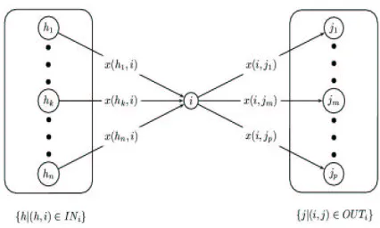
Figure 1: An illustration of flow entering and exiting node..

bined incoming flow, /1032457698;:=<?>*@BAC D, from the

entering edges EDF, as well as the combined

outgo-ing flow, / 0G54H6B8JI+KJLM> *@N POQ , via the exiting edges RTSVU

F. (See Figure 1.) If a feasible solution can be

found, the net flow (the difference between the en-tering and exiting flow) at each node must fulfill the corresponding supply or demand requirement.

Formally, the MCF problem can be stated as:

Minimize WMXNY Z;[J\ ]

^`_bacdfehgji

X

.Bk=l [ mDZ

X

.Bk7l

[

(1)

subject to

]

^`_bacdfenQoqpNr

Z

X

.Bk7l [ts ]

^vuwa_Gdfeyx3zqr

Z

X7{ kB.

[|\~}

X

.

[

k;.|€‚ (2)

Z

X

.Bkfl [„ƒ†…

k9

X

.Bkfl

[

€ˆ‡ (3)

The constraint specified by (2) ensures that the dif-ference between the flow entering and exiting each node matches its supply or demand exactly.

The next constraint (3) ensures that the flow is trans-ported from the supply to the demand but not in the opposite direction. Finally, selecting route‰ POQ

requires a transportation “effort” of ;N POŠ (cost

of the route) multiplied by the amount of supply transported *@N POQ (the term inside the summation

in eqn. (1)). Taking the summation of the effort,

;N POQŒ‹y*j‰ POQ, of cheapest routes yields the desired

distance between the supply and the demand.

2.2 Semantic Distance as MCF

demand. The cost of the routes between nodes is determined by a semantic distance measure defined over any two nodes in the ontology. Now, as in the grocery delivery domain, the goal is to find the MCF from supply to demand.

We can treat any ontology as the transport net-work. A relation (such as hyponymy) between two concepts andO is represented by an edgeN POQ , and

the cost on each edge can be defined as the

tic distance between the two concepts. This seman-tic distance can be as simple as the number of edges separating the concepts, or more sophisticated, such as Lin’s (1998) information-theoretic measure. (See Budanitsky and Hirst (2006) for a survey of such measures).

Numerous methods are possible for converting the word frequency vector of a context to a concept frequency vector (i.e., a context profile). One simple method is to transfer each element in the word vector (i.e., the frequency of each word) to the correspond-ing concepts in the ontology, resultcorrespond-ing in a vector of concept frequencies. In this paper, we have cho-sen a uniform distribution of word frequency counts among concepts, instead of a weighted distribution towards the relevant concepts for a particular text. Since we wish to evaluate the strength of our method alone without any additional NLP effort, we bypass the issue of approximating the true distribution of the concepts via word sense disambiguation or class-based approximation methods, such as those by Li and Abe (1998) and Clark and Weir (2002).

To calculate the distance between two profiles, we need to cast one profile as the supply ( ) and the

other as the demand (Ž ). Note that our distance

is symmetric, so the choice of the supply and the demand is arbitrary. Next, we must determine the value of at each concept node ; this is just

the difference between the (normalized) supply fre-quencyN‘’“ and demand frequency‰”•’D :

}

X

.

[|\—–˜ X9™

[ s‚–Bš X9™

[

(4)

This formula yields the net supply/demand, , at

node. Recall that our goal is to transport all the

sup-ply to meet the demand—the final step is to deter-mine the cheapest routes between andŽ such that

the constraints in (2) and (3) are satisfied. The total distance of the routes, or the MCF,›Jqœ*„ in eqn. (1),

is the distance between the two context profiles.

Finally, it is important to note that the MCF for-mulation does not simply find the shortest paths from the concept nodes in the supply to those in the demand. Because a profile is a frequency-weighted concept vector, some concept nodes are weighted more heavily than others, and the routes between such nodes across the two profiles are also weighted more heavily. Indeed, in eqn. (1), the cost of each route,‰ POQ, is weighted by*@N POQ (how much

sup-ply, or frequency weight, is transported between nodes andO ).

3 Graphical Issues

As alluded to in the introduction, certain concept-to-concept distances pose a problem to solving the MCF problem easily. The details are described next.

3.1 Additivity

In theory, our method has the flexibility to incorpo-rate different concept-to-concept distances. The is-sue lies in the algorithms for solving MCF problems. Existing algorithms are greedy—they take a step-wise “localist” approach on the set of edges connect-ing the supply and the demand; i.e., at each node, the cheapest outgoing edge is selected. The assump-tion is that the concept-to-concept distance funcassump-tion is additive. Mathematically, for any path from node

to node ,žQbOqŸ; PO w y¡y¡y¡¢ qbOy£Q¤C q POy£|‰¥ , wherej¦OqŸ

and §¨O £ , the distance between nodes and  is

the sum of the distance of the edges along the path:

©

™«ª¬­X9™ k®

[|\°¯w± ²]

³|´tµ

©

™«ª¬­X·¶

³

k

¶

³|¸

²

[

(5)

The additivity of a concept-to-concept distance en-tails that selecting the cheapest edge at each step (i.e., locally) yields the overall cheapest set of routes (i.e., globally). Note that some of the most success-ful concept-to-concept distances proposed in the CL literature are non-additive (e.g., Lin, 1998; Resnik, 1995). This poses a problem in solving our network flow problem—the global distance between any con-cepts, and , cannot be correctly determined by the

greedy method.

3.2 Constructing an Equivalent Bipartite Network

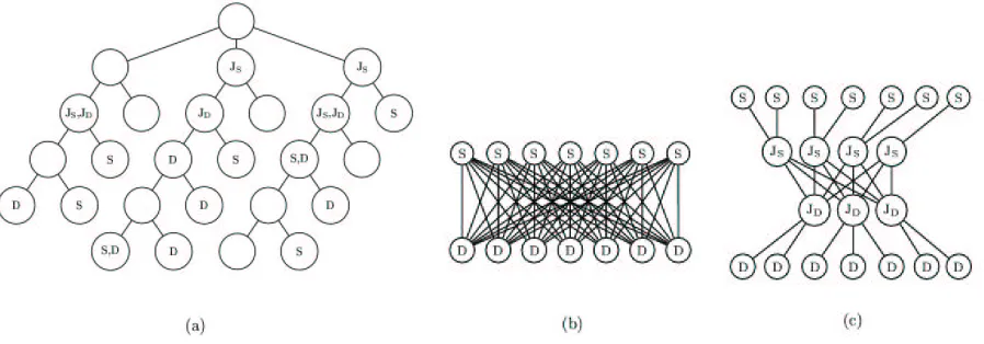
Figure 2: An illustration of the transformations (left to right) from the original network (a) to the bipartite network (b), and finally, to the network produced by our transformation (c), given two profiles S and D. Nodes labelled with either “S” or “D” belong to the corresponding profile. Nodes labelled with “¹»º ” or “¹y¼ ” are junction nodes (see section 4.2).

of the network into a new network such that the concept-to-concept distance is preserved, but with-out the problem introduced by non-additivity. One possible solution is to construct a complete bipar-tite graph between the supply nodes and the demand nodes (the nodes in the two context profiles). We set the cost of each edge B½¾ N¿Š in the bipartite graph to

be the concept-to-concept distance between½ and ¿

in the original network. Since there is exactly one edge between any pair of nodes, the non-additivity is removed entirely. (See Figures 2(a) and 2(b).) Now, we can apply a network flow solver on the new graph.

However, one problem arises from performing the above mapping—there is a processing bottleneck as a result of the quadratic increase in the number of edges in the new network. Unfortunately, though tractable, polynomial complexity is not always prac-tical. For example, with an average of 900 nodes per profile, making 120 profile comparisons in addi-tion to network re-structuring can take as long as 10 days.2 If we choose to use a non-additive distance, the method described above does not scale up well for a large number of comparisons. Next, we present a method to alleviate the complexity issue.

4 Network Transformation

One method of alleviating the bottleneck is to reduce the processing load from generating a large number

2_{This is tested on a context comparison task not reported in}

this paper. The code is scripted in perl. The experiment was performed on a machine with two P4 Xeon CPUs running at 3.6GHz, with a 1MB cache and 6GB of memory.

of edges. Instead of generating a complete bipar-tite network, we generate a network which approx-imates both the structure of the original network as well as that of the complete bipartite network. The goal is to construct a pared-down network such that (a) a reduction in the number of edges improves effi-ciency, and (b) the resulting distance distortion does not hamper performance significantly.

4.1 Path Shape in a Hierarchy

To understand our transformation method, let us fur-ther examine the graphical properties of an ontology as a network. In a hierarchical network (e.g., Word-Net, Gene Ontology, UMLS), calculating the dis-tance between two concept nodes usually involves travelling “up” and “down” the hierarchy. The sim-plest route is a single hop from a child to its parent or vice versa. Generally, travelling from one node

to another nodeO consists of an A-shaped path

as-cending from node to a common ancestor of and

O , and then descending to nodeO .

Interestingly, our description of the A-shaped path matches the design of a number of concept-to-concept distances. For example, distances that in-corporate Resnik’s (1995) information content (IC),

À~ÁbÂ;Ã

fÄÅDƉÇ;ÈÉÆÊÄ?ËND , such as those of Jiang and

Con-rath (1997) and Lin (1998), consider both the (low-est) common ancestor as well as the two nodes of interest in their calculation.

The complete bipartite graph considered in sec-tion 3.2 directly connects each node s in profile 

to node ¿ in profile Ž , eliminating the typical

non-additivity issue, by generating an edge with the exact concept-to-concept distance for each potential node comparison, but, as noted above, is too inef-ficient. Our solution here is to construct a network that uses the idea of a pared-down A-shaped path to mostly avoid non-additivity, but without the ineffi-ciency of the complete bipartite graph. Thus, as ex-plained in more detail in the following subsections, we trade off the exactness of the distance calculation against the efficiency of the network construction.

4.2 Network Construction

In our network construction, we exploit the general notion of an A-shaped path between any two nodes, but replace the “tip” of the A with two nodes. Then for each node½ and ¿ in profiles  andŽ , we

gen-erate an edge from s to an ancestor ÌJÍ of ½ (the

left “branch” of the A), an edge from d to an an-cestor̊Πof ¿ (the right “branch” of the A), and an

edge betweenÌtÍ and̊Π(the two nodes forming the

“elongated tip” of the A). Each edge has the exact concept-to-concept distance from the original net-work, so that the distance between any two nodes

½ and¿ is the sum of three exact distances.

The set of ancestor nodes,Ì|Í and̊Π, comprise the

“junction” points at which the supply from can be

transported across to the nodes in Ž to satisfy their

demand. The set of junction nodes, Ï Ð , for a

pro-file Ñ , must be selected such that for each node

in Ñ , ϾРcontains at least one ancestor of . (See

section 4.4 for details on the junction selection pro-cess.) The resulting network is constructed by di-rectly connecting each profile to its corresponding junction, then connecting the two junctions in the middle (Figure 2(c)).

The difference between the complete bipartite network and the transformed network here is that, instead of connecting each node in  to every node

in Ž , we connect each node in ÏtÒ to every node

in ÏQÓ . Compare the transformed network in

ure 2(c) with the complete bipartite network in Fig-ure 2(b). The complete bipartite component in the transformed network (the middle portion between the junction nodes labelled Ï Ò and ÏŠÓ ) is

consid-erably smaller in size. Thus, the number of edges in the transformed network is significantly fewer as well.

Next, we can proceed to define the cost function

on the transformed network. Observe that each edge

B½¾ N¿Š , with cost ԒfÕhËy­Õ qÔ| , in the complete bipartite

network, where½~ ,¿Ö†Ž , is now instead

repre-sented by three edges: ­Õ; q×;Øy,D×Ø» q×ÙÚ , and D×;ÙQ qÔ|,

where× Ø ÛÏQÒ and ×;ÙTÛÏ Ó . Thus, the transformed

distance between½ and¿ , ԒfÕhËBÜ«ÝfÞDßyØ¢­Õ; qÔ| , becomes:

© ™«ª¬3à·á3â ¯­ã X9ª k © [|\ © ™«ª¬X9ª k‰ä ã [Qå © ™«ª¬­X ä ã k‰ä‰æ [Qå © ™3ªP¬­X äæyk © [ (6)

where ¿Ú½»çyN POQ is the precise concept-to-concept

distance between and O in the original network.

Once we have set up the transformed network, we can solve the MCF in this network, yielding the dis-tance between the two (supply and demand) profiles.

4.3 Distance Distortion

Because the distance between nodes½ and ¿ is now

calculated as the sum of three distances (eqn. (6)), some distortion may result for non-additive concept-to-concept distances. To illustrate the distortion ef-fect, consider Jiang and Conrath’s (1997) distance:

© ™«ª¬èbéDX9™ k ¶ [|\ëê‰ì X9™ [Úå†ê‰ì X·¶ [Qsîíê‰ì Xfï ìtð X9™ k ¶ [B[ (7)

where Eñ’“ is the information content of a node

, and òVñjóô’‰ BõŠ is the lowest common subsumer

of nodes and O . This distance measures the

dif-ference in information content between the concepts and their lowest common subsumers.

After the transformation, the distance is distorted in the following way. If and O have no common

junction ancestor, then Ԓ=ÕwËvöP÷ à·á«â

¯Pã

’ BõŠ becomes:

©

™«ª¬èbébøùvúGûfü‰X .Bkfl

[!\ ýê‰ì X9™ [Úåþê‰ì X ä > [ sîíê‰ì X ä > [=ÿ»å ýê‰ì X·¶ [;åþê‰ì X ä è [ sþí‰ê‰ì X ä è [=ÿ»å ýê‰ì X ä >[¾åþê‰ì X ä è [tsîíê‰ì Xfï ìtð X ä > kNä è [B[=ÿ \ ê‰ì X9™ [Úåîê‰ì X·¶ [Šsþíê‰ì Xfï ìtð X ä > kNä è [B[ (8) where Ì 5 and Ì

H are the junction ancestors of

and O , respectively. Otherwise, if and O

share a common ancestor Ì at the junction, then

Ԓ=ÕwË·öP÷ à·á«â

¯Pã

’‰ BõŠ becomes Eñ’“ Eñ3õŠ À

EñD׊ ,

where the term

Eñ ò ñjó D×;F“ q×NöMD in eqn. (8) is

re-placed by

EñD׊ . In either case, the transformation

replaces the lowest common subsumer òVñjóô’‰ BõŠ

in eqn. (7) with some other common subsumer

ñjó ’ BõŠ (òVñjóôD× F q× ö orÌ , mentioned above).

Un-less ñjó ’ BõŠŒ¨ò ñjó ’ BõŠ , the distance is distorted

by using a less precise quantity,Eñ yñjóô’‰ BõŠD .

its frequency in a large corpus. An increment in the frequency of a concept leads to an increment in the frequency of all its ancestors. Due to the frequency percolation, concepts with a small depth tend to ac-cumulate higher counts than those deeper in the hi-erarchy (note the difference in depth: ԾʭÄ?Ë



0

F

4

ö

6

ÔQÊ­Ä?Ë 

0

F

4

ö

6). Thus, we expect the

informa-tion content of a concept to be higher than its an-cestors, i.e., a concept is more semantically specific than its ancestors, which is captured by the use of the negative Á7Â;Ã

function in the definition of IC. The transformed distance is distorted accordingly (Eñ yñjóô’‰ BõŠD

EñòVñjóô’‰ BõŠD ).

4.4 Junction Selection

Selection of junction nodes is a key component of the network transformation. Trivially, a junction consisting of profile nodes yields a network equiva-lent to the complete bipartite network. The key is to select a junction that is considerably smaller in size than its corresponding profile, hence, cutting down the number of edges generated, which results in sig-nificant savings in complexity.

Note that there is a tradeoff between the over-all computational efficiency and the similarity be-tween the transformed network and the complete bi-partite network. The closer the junctions are to the corresponding profiles, the closer the transformed network resembles the complete bipartite network. Though the distance calculation is more accurate, such a network is also more expensive to process. On the other hand, there are fewer nodes in a junc-tion as it approaches the root level, but there is more distortion in the transformed concept-to-concept dis-tance. Clearly, it is important to balance the two fac-tors.

Selecting junction nodes involves finding a smaller set of ancestor nodes representing the pro-file nodes in a hierarchy. In other words, the junc-tion can be viewed as an alternative representajunc-tion which is a generalization of the profile nodes. In addition to the profile nodes, the junction nodes are also included in the transformed network. They may provide extra information about the corresponding context.

Finding a generalization of a profile is explored in the works of Clark and Weir (2002) and Li and Abe (1998). Unfortunately, the complexity of these

algo-rithms is quadratic (the former) or cubic (the latter) in the number of nodes in a network, which is unac-ceptably expensive for our transformation method. Note that to ensure every profile node has an ances-tor node in the junction, the selection process has a linear lower bound. To keep the cost low, it is best to keep a linear complexity for the junction selection process. However, if this is not possible, it should be significantly less expensive than a quadratic com-plexity. We will empirically explore the process fur-ther in section 5.3.

5 Context Comparison

As alluded to earlier, our network flow method pro-vides an alternative to a purely distributional and non-graphical approach to context comparison. In this paper, we will test both variants of our method (with or without the transformation in section 4) in a name disambiguation task in which the context words within a small window surrounding the am-biguous words are compared. Our preliminary anal-ysis shows that our general network flow framework is robust and efficient.

5.1 Name Disambiguation

The goal for name disambiguation is to classify each ambiguous instance on the basis of its surrounding context. One approach is to use an unsupervised method such as clustering. This involves making a large number of pairwise comparisons between in-dividual contexts. Given that there is an overhead to incorporating ontological information, our net-work flow method does not compute distances as ef-ficiently as calculating a purely arithmetic distance such as cosine or Euclidean distance. Our alterna-tive approach is to use minimal training data. Us-ing a handful of contexts, we can build a “gold stan-dard” profile for each sense of an ambiguous name by using the context words of a small number of instances. We then compare the context profile of each instance to the gold standards. Each instance is given the label of the gold standard profile to which its context profile is the closest.

5.2 Experimental Setup

Name Pairs Baseline 200 (Full) 200 (Trans) 100 (Full) 100 (Trans)

Ronaldo/David Beckham 0.69 0.80 0.88 0.79 0.84

Tajik/Rolf Ekeus 0.74 0.97 0.99 0.98 0.99

Microsoft/IBM 0.59 0.73 0.75 0.73 0.71

Shimon Peres/Slobodan Milosevic 0.56 0.96 0.99 0.97 0.99

Jordan/Egyptian 0.54 0.77 0.76 0.74 0.76

Japan/France 0.51 0.75 0.82 0.75 0.83

Weighted Average 0.53 0.77 0.82 0.76 0.82

Table 1: Name disambiguation results (accuracy/F-measure) at a glance. The baseline is the relative frequency of the majority name. “200” and “100” give the averaged results (over five different runs) using 200 and 100 randomly selected training instances per ambiguous name. The weighted average is calculated based on the number of test instances per task. “Full” and “Trans” refer to the results using the full network (pre-transformation) or the pared-down network (with transformation), respectively.

the Agence France Press English Service portion of the GigaWord English corpus distributed by the Lin-guistic Data Consortium. It consists of the contexts of six pairs of names, including: the names of two soccer players (Ronaldo and David Beckham); an ethnic group and a diplomat (Tajik and Rolf Ekeus); two companies (Microsoft and IBM); two politicians (Shimon Peres and Slobodan Milosevic); a nation and a nationality (Jordan and Egyptian); and two countries (France and Japan). These name pairs are selected by Pedersen et al. (2005) to reflect a range of confusability between names.

Each pair of names serves as one of six name disambiguation tasks. Each name instance con-sists of a context window of 50 words (25 words to the left and to the right of the target name), with the target name obfuscated. For example, for the task of distinguishing “David Beckham” and “Ronaldo”, the target name in each instance be-comes “David BeckhamRonaldo”. The goal is to recover the correct target name in each instance.

5.3 Junction Selection

We reported earlier that a complete bipartite graph with 900 nodes is too expensive to process. Our first attempt is to select a junction on the basis of the number of nodes it contains. Here, the junctions we select are simple to find by taking a top-down ap-proach. We start at the top nine root nodes of Word-Net (nodes of zero depth) and proceed downwards. We limit the search within the top two levels because the second level consists of 158 nodes, while the fol-lowing level consists of 1307 nodes, which, clearly, exceeds 900 nodes. Here, we select the junction which consists of eight of the top root nodes (sil-bings of entity) and the children of entity, given that

entity is semantically more general than its siblings.3

In our current experiment, we use Jiang and Conrath’s distance for its ease of analysis. As shown in section 4.3, only one term in the distance,

EñòVñjó ’ BõŠD , is replaced because of the use of the

junction nodes. Any change in the performance (in comparison to our method without the transforma-tion) can be attributed to the distance distortion as a result of this term being replaced. The analysis of experimental results (next section) is made easy because we can assess the goodness of the trans-formation given the selected junction—a significant degradation in performance is an indication that the junction nodes should be brought closer to the pro-file nodes, yielding a more precise distance.

6 Results and Analysis

To compare the two variants of our method, we perform our name disambiguation experiment us-ing 100 and 200 trainus-ing instances per ambiguous name to create the gold standard profiles. See Ta-ble 1 for the results. Comparing the results using the full network and the transformed network, ob-serve that there is very little performance degrada-tion; in fact, in most cases, there is an increase in accuracy (the difference is significant, paired t-test with % ¡`% ).

Distance Transformation In Jiang and Conrath’s formulation, the network transformation replaces the term

Eñ ò ñjó ’‰ Bõ D with

Eñyñjó ’‰ Bõ D ,

where ñjó ’ BõŠ is some common ancestor of and

3

O , whose depth is small. Junction nodes with a small

depth distort the distance more than those with a larger depth. Surprisingly, our experiment indicates that using such nodes produces equally good or bet-ter performance. This suggests that selecting a junc-tion with a larger depth, at least for the data in this task, is not necessary.

Speed Improvement In comparison to our re-ported running time on the pre-transformation net-work (120 comparisons running for 10 days), on the same machine, making 12,000 comparisons can now be accomplished within two hours. In terms of complexity, if we have profile nodes and O

junc-tion nodes, the number of edges to be processed is

Oq . Given that our junctions have

signif-icantly fewer nodes than the original profiles, the running time is significantly less than quadratic in the number of profile nodes.

7 Conclusions

We have given an overview of our network flow for-malism which seamlessly combines distributional and ontological information. Given a suitable on-tology, a context vector of word frequencies can be transformed into a context profile—a frequency distribution over the concepts in the ontology. In contrast to traditional non-graphical approaches to measuring only the distributional distance between context vectors, we provide a graphical formalism which incorporates both the semantic distance of the component nodes as well as the distributional differ-ences between the context profiles. By taking advan-tage of the graphical structure of an ontology, our method allows a systematic and meaningful way of abstracting over words in a context, and by exten-sion, a meaningful way of comparing contexts.

One concern with our method in its pre-transformation form is its inability to incorporate sophisticated concept-to-concept semantic distances efficiently. To remedy this, we propose a novel tech-nique that mimics the structure of the more compu-tationally intensive network. Our preliminary eval-uation shows that the transformation does not ham-per the method’s ability to make fine-grained seman-tic distinctions, and the computational complexity is drastically reduced as well. Generally, our network flow method presents a highly competitive

alterna-tive to a purely distributional and non-graphical ap-proach.

In our on-going work, we are further exploring how the choice of junction influences the perfor-mance of different types of concept-to-concept se-mantic distances. For example, would a bottom-up junction selection approach (from the profile nodes instead of from the root level) result in better per-formance? In addition, we intend to examine the graphical properties of the individual profiles as well as the routes between the concepts across profiles selected by our network flow methods. Such analy-ses will help us gain insight into the strengths (and weaknesses) of taking advantage of a graphical rep-resentation of contexts as well as treating an ontol-ogy as a metric space for context comparisons.

References

Budanitsky, A. and Hirst, G. (2006). Evaluating WordNet-based measures of semantic distance. Computational Linguistics. To appear.

Clark, S. and Weir, D. (2002). Class-based probability estima-tion using a semantic hierarchy. Computaestima-tional Linguistics, 28(2):187–206.

Jiang, J. and Conrath, D. (1997). Semantic similarity based on corpus statistics and lexical taxonomy. In Proceedings on the International Conference on Research in Computational Linguistics, pages 19–33.

Li, H. and Abe, N. (1998). Word clustering and disambiguation based on co-occurrence data. In Proceedings of COLING-ACL 1998, pages 749–755.

Lin, D. (1998). An information-theoretic definition of similar-ity. In Proceedings of International Conference on Machine Learning.

Mihalcea, R. (2006). Random walks on text structures. In Pro-ceedings of CICLing 2006, pages 249–262.

Miller, G. A. and Charles, W. G. (1991). Contextual correlates of semantic similarity. Language and Cognitive Processes, 6(1):1–28.

Navigli, R. and Velardi, P. (2005). Structural semantic inter-connections: A knowledge-based approach to word sense disambiguation. IEEE Transactions on Pattern Analysis and Machine Intelligence, 27(7).

Pedersen, T., Purandare, A., and Kulkarni, A. (2005). Name discrimination by clustering similar context. In Proceedings of the Sixth International Conference on Intelligent Text Pro-cessing and Computational Linguistics.

Resnik, P. (1995). Using information content to evaluate se-mantic similarity in a taxonomy. In Proceedings of the 14th International Joint Conference on Artificial Intelligence. Sch¨utze, H. (1998). Automatic word sense discrimination.

Computational Linguistics, 24(1):97–123.