Compressed Sensing for Fast Electromagnetic Scattering Analysis
of Complex Linear Structures
Xuehua Ma1, Mingsheng Chen2, *, Jinhua Hu2, Meng Kong2, Zhixiang Huang1, and Xianliang Wu1, 2
Abstract—When method of moments (MOM) is applied to calculate electromagnetic scattering problems of the linear structures, traditional basis functions such as RWG functions are unable to satisfy the requirements of numerical discretization, so linear basis functions are constructed to discrete line structures. To avoid direct calculation of dense impedance matrix equation, compressed sensing (CS) in conjugation with appropriate transformation is introduced. Firstly, the impedance matrix equation is operated to obtain an alternative equation in transform domain. Secondly, CS is used to form an underdetermined equation to be solved, under the theoretical framework of CS, and the underdetermined equation can be solved by reconstruct algorithm but not iterative approach. Finally, numerical simulations of single wound axial mode helical antenna and four element linear antennas array are discussed to demonstrate the efficiency and accuracy of the proposed method.
1. INTRODUCTION
With the rapid development of wireless communication narrow-pulse radar technology and electromagnetic compatibility/electromagnetic interference (EMC/EMI), electromagnetic scattering problems of thin-line antennas and linear structures [1–3] have attracted a great deal of attention owing to their wide applications. Among various numerical methods for analysis of electromagnetic scattering and radiation problems, the method of moments (MOM) is widely used due to its accuracy [4].
When the method of moments is used to solve surface integral equations to accomplish the electromagnetic scattering analysis of differently shaped conductors, the first step is to discretize the surface currents of the target, and then proper basis functions are constructed to expand the surface currents. Finally, a matrix equation is formed into testing techniques such as Galerkin method and point match method.
Currently, for common three-dimensional objects, Rao-Wilton-Glisson (RWG) basis functions [5] are usually used to expand surface currents. However, when the targets of line structures are considered, the RWG basis function is constrained by the target structure and cannot meet the requirements of the discretization. Therefore, the line basis function [6] is introduced to spatially discretize the line structure targets.
Meanwhile, to ensure the accuracy of calculation, the traditional method of moments is always used on the basis of a full coupling model in which all the interaction between field points and source points must be considered. Then a dense impedance matrix will be generated, and the memory consumption computational complexity will be unsatisfactory. To avoid this situation, sparse transform techniques mentioned in [7–10] are used to obtain an alternative equation for MOM. Then the compressed sensing theory [11–14] is introduced, and several rows of the impedance matrix in transform domain are extracted
Received 13 November 2018, Accepted 23 January 2019, Scheduled 10 February 2019
* Corresponding author: Mingsheng Chen ([email protected]).
1 School of Electronic and Information Engineering, Anhui University, Hefei, China. 2 Anhui Key Laboratory of Emulation and
to form an undermined low dimension matrix equation, with the help of reconstruct algorithms instead of iterative approach. The current coefficients can be computed, and the amount of memory consumption and computational efficiency can be improved greatly.
2. ALGORITHM THEORY
2.1. Numerical Discretization of Electric Field Integral Equation for Linear Structure Target
The expression of the electric field integral equation of the linear structure target is as follows:
jkη
l
J(r)G(r,r) + 1
k2∇·J(r
)∇G(r,r)dl=Einc(r) (1)
where J(r) denotes the unknown surface current density, k0 the free-space wave number, η0 the free-space wave impedance, and G(r, r) the well-known free-space Green’s function. The surface current density can then be expanded using linear vector basis functions as
J(r, t)≈
Nw
n=1
InfnW(r) (2)
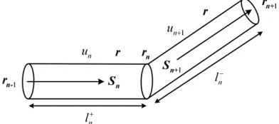
In whichfnW is defined on two continuous straight segments that are denoted byunandun+1, as shown in Fig. 1. The equivalent method can keep the continuity of the current on the wire, and fnW is given by
fnW(r) =
⎧ ⎨ ⎩
Sn|r−rn−1|/|rn−rn−1| r∈un Sn+1(1− |r−rn|/|rn+1−rn| r∈un+1)
0 elsewhere
. (3)
Here,Sn= (rn−rn−1)/|rn−rn−1|is the axial unit vector of theun line segment.
Figure 1. The linear vector basis functions.
Substituting Eqs. (2), (3) into Eq. (1) and applying Galerkin’s method to Eq. (1) gives the following equations
Z(k)·I(k) =V(k) (4)
Here,Z(k) is the impedance matrix, V(k) the excitation column vector, andI(k) the unknown vector current to be solved. Z(k) and V(k) are given by
Z(k)mn = jωμ
l
l
fmw(r)·fnw(r)G(r,r)dldl−
j ωμ
l
l
∇ ·fmw(r)∇·fnw(r)G(r,r)dldl (5)
V(k)m =
lf w
where m and n are corresponding to the index of the line base function and the index of the test function, respectively. The expansion of the first term in Equation (5) with the linear basis function fnW yields:
l
l
fmw(r)·fnw(r,)G(r, r,)dldl=
l+m
l+n
|r−rm−1|
|rm−rm−1|2
|r−rn−1|
|rn−rn−1|2
(rm−rm−1)·(rn−rn−1)
G(r, r)dldl+
l+m
l−n
|r−rm−1|
|rm−rm−1|2
|rn+1−r|
|rn+1−rn|2
(rm−rm−1)·(rn+1−rn)
G(r, r)dldl+
l− m l+ n
|rm+1−r|
|rm+1−rm|2
|r−rn−1|
|rn−rn−1|2
(rm+1−rm)·(rn−rn−1)
G(r, r)dldl+
l− m l− n
|rm+1−r|
|rm+1−rm|2
|rn+1−r|
|rn+1−rn|2
(rm+1−rm)·(rn+1−rn)
G(r, r)dldl (7)
The integral expansion in the second item of formula (5) results in:
l
l
∇·fnw(r)∇ ·fmw(r)G(r, r)dldl
= 1
|rm−rm−1| 1
|rn−rn−1|
l+m
l+n
G(r, r)dldl−
1
|rm+1−rm| 1
|rn−rn−1|
lm−
l+n
G(r, r)dldl−
1
|rm−rm−1| 1
|rn+1−rn|
l+ m l− n
G(r, r)dldl+
1
|rm+1−rm| 1
|rn+1−rn|
lm−
l−n
G(r, r)dldl (8)
2.2. Discrete Sparse Transformation and Prior Knowledge Extraction The original moment Equation (4) can be expressed as
⎡ ⎢ ⎢ ⎢ ⎢ ⎢ ⎢ ⎢ ⎣
Z11 Z12 · · · Z1N
Z21 Z22 · · · Z2N
· · · · · · · · · · ··
ZN1 ZN2 · · · ZNN
⎤ ⎥ ⎥ ⎥ ⎥ ⎥ ⎥ ⎥ ⎦ ⎡ ⎢ ⎢ ⎢ ⎢ ⎢ ⎢ ⎢ ⎣ I1 I2 · · · IN ⎤ ⎥ ⎥ ⎥ ⎥ ⎥ ⎥ ⎥ ⎦ = ⎡ ⎢ ⎢ ⎢ ⎢ ⎢ ⎢ ⎢ ⎣ V1 V2 · · · VN ⎤ ⎥ ⎥ ⎥ ⎥ ⎥ ⎥ ⎥ ⎦ (9)
The sparse transformations can be operated by ˜Z = W ZWH, ˜I = W I, ˜V = W V, where W is the orthogonal matrices constructed by discrete sparse transform and W WH = U, WH the conjugate transposed matrix ofW, andU the identity matrix. Equation (4) can be transformed into the following matrix equation
˜
The threshold is σ in transform domain and is defined as
σ=τZ˜1/N =τ ·maxm
n
˜Z(m, n)/N (11)
whereN is the dimension of the matrix, andτ is the control variable to decide the sparsity of impedance matrix in transform domain. The matrix element will be approximately set to zero as it is below this threshold.
According to Equation (10), ˜V is the excitation vector in transform domain, and it is also a sparse vector after thresholding operation. For the same linear system, the vector ˜I is also a sparse vector that is high relevant to ˜V. The position of the line is equally important. Therefore, onlyM rows of the same important position in ˜V and ˜Z are extracted, and the small-scale matrices ˜VMCS×1 and ˜ZMCS×N are formed respectively. Equation (10) becomes an underdetermined equation:
˜
ZCSM×N˜IN×1 =V˜MCS×1 (M << N) (12) From the view point of theoretical framework of compressed sensing that is described in [11–13], ˜
VCSM×1 can be considered as a measured value, and ˜ZMCS×N is the measurement matrix.
Instead of the traditional iteration method, the problem can be solved by the OMP technique which is described in [13, 15].
The real current coefficient vector IN×1 is obtained by inverse transform.
IN×1 =WN−×1N ·I˜N×1 (13) The Discrete Wavelet Transform (DWT) is used as a sparse transform for scattering analysis of bodies of revolution in [16]. After setting the appropriate threshold and extraction, it can be solved by the above method. As other techniques such as Discrete Cosine Transform (DCT) and Discrete Fourier Transform (DFT) are used to construct the sparse matrix, this method is still applicable. It can be seen that as long as the appropriate sparse basis is selected, the method can be used to efficiently obtain the results.
In this paper, considering the special structure of linear antennas, we use the Discrete Fourier Transform (DFT) to form a sparse transform. After setting the threshold in the sparse domain and extraction, the obtained equation also satisfies the theory of compressed sensing.
The Discrete Fourier Transform (DFT) can be described as follows:
X[k] =
N−1
n=0
x[n]e−j2π·Nk·n=
N−1
n=0
x(n)Tnkn k= 0,1,· · ·N −1, TN =e−j2π/N (14)
And the matrix form can be expressed as follows
⎡ ⎢ ⎢ ⎢ ⎢ ⎢ ⎢ ⎢ ⎢ ⎢ ⎢ ⎣ X(0) X(1) X(2) · · ·
X(N−1)
⎤ ⎥ ⎥ ⎥ ⎥ ⎥ ⎥ ⎥ ⎥ ⎥ ⎥ ⎦ = ⎡ ⎢ ⎢ ⎢ ⎢ ⎢ ⎢ ⎢ ⎢ ⎢ ⎢ ⎢ ⎣
1 1 1 · · · 1
1 TN1 TN2 · · · TNN−1
1 TN2 TN4 · · · TN2(N−1)
· · · · · · · · · · · · · · ·
1 TNN−1 TN2(N−1) · · · TN(N−1)(N−1)
⎤ ⎥ ⎥ ⎥ ⎥ ⎥ ⎥ ⎥ ⎥ ⎥ ⎥ ⎥ ⎦ ⎡ ⎢ ⎢ ⎢ ⎢ ⎢ ⎢ ⎢ ⎢ ⎢ ⎢ ⎣ x(0) x(1) x(2) · · ·
x(N −1)
⎤ ⎥ ⎥ ⎥ ⎥ ⎥ ⎥ ⎥ ⎥ ⎥ ⎥ ⎦ (15)
3. NUMERICAL EXAMPLES
Example 1. A single-wound axial helical antenna was tested with its radius of 0.5 m, helix angleα= 20◦ and each pitch of 1.143 m with 10 turns. The entire antenna height is 11.43 m, and the wire radius is 0.003 m. The physical structure is shown in Fig. 2.
Figure 2. The axial mode helical antenna.
Figure 3. The nonzero elements distribution in vector ˜V for the single-wound axial helical antenna.
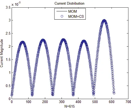
incident wave illuminated at angle of θ = 50◦, ϕ= 60◦, the matrix equations are sparse by using the Discrete Fourier Transform (DFT) under the MOM calculation framework. In the sparse domain, the threshold of the excitation vector is set to 0.002, and the number of non-zero elements is K = 212. Fig. 3 shows the numerical distribution of the excitation vectors after setting the threshold in the sparse transform domain. The blue part indicates the nonzero part and is used to restore the original current. It can be regarded as a priori knowledge for the proposed method to lock and extract the position of a specific row from impedance matrix ˜Z, which will construct a measurement matrix ˜ZMCS×N. In the impedance matrix, threshold is set to 0.2, which corresponds toM =K= 212 to construct a small-scale matrix as shown in Fig. 4. In the impedance matrix, the number of non-zero elements is 609978. The small-scale matrix after extraction is shown in Fig. 4, and the number of non-zero elements is reduced to 136471, a decrease of 77.6% compared with the original matrix. The comparison results of the current sparse solutions obtained by MOM and the CS technique are shown in Fig. 5. It can be seen that they agree well with each other.
Figure 4. The low dimension impedance matrix extracted for the single-wound axial helical antenna.
Figure 5. The current of the single-wound axial helical antenna computed by direct MOM solution and CS method.
Figure 6. The model of an antenna array.
each unit antenna and the spacing between the elements are λ/2, and the radius of a single antenna is 0.002 m. The working model is shown in Fig. 6.
Figure 7. The nonzero element distribution in vector ˜V for the antenna array.
Figure 8. The low dimension impedance matrix extracted the antenna array.
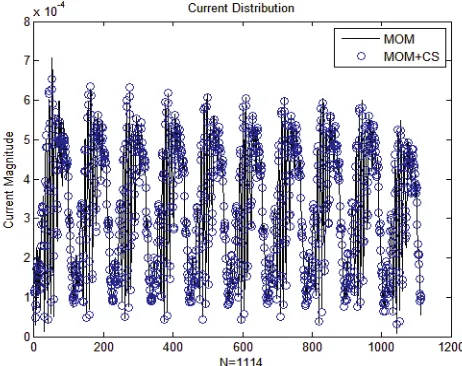
Figure 9. The currents of the antenna array computed by direct MOM solution and CS method.
set to 0.005, which corresponds to M = K = 190 is set to construct a small-scale matrix as shown Fig. 8. In the impedance matrix, the number of non-zero elements is 76241. In the small-scale matrix, the number of non-zero elements is reduced to 23966, and there is a decrease of 68.6% compared with the original matrix. The comparison results of the current sparse solutions obtained by MOM and the CS technique are shown in Fig. 9.
4. SUMMARY
In this paper, the linear basis function is applied to solve the linear structure electric field integral equation, and the detailed expansion formula and solution process of the linear basis function in the electric field integral equation are deduced. In addition, a new method formed by compressed sensing and sparse matrix transform is introduced to make the impedance matrix sparse to further improve the computational efficiency. Two kinds antenna structures are analyzed, and the results of the surface current obtained by the proposed method agree well that of MOM.
ACKNOWLEDGMENT
This work was supported by the National Natural Science Foundation of China (51477039, 61801163), the National Natural Science for Excellent Young Scholars (61722101), and the Key Projects of Natural Science Research under Grant KJ2015A260 of Anhui.
REFERENCES
1. Xu, X. W., B. Huo, and M. He, “Exact modeling for the influence of the von karman radome on antennas,”Transactions of Beijing Institute of Technology, 532–535, Beijing, China, 2006.
2. Zhao, W. J. and L. W. Li, “Efficient analysis of antenna radiation in the presence of airborne dielectric radomes of arbitrary shape,” IEEE Transaction on Antennas and Propagation, Vol. 53, 32–35, 2005.
3. Ma, Y., “Characteristic analysis of several wire antennas attached to an arbitrary faceted conducting body,” University of Electronic Science and Technology, Chengdu, China, 2002. 4. Harrington, R. F., Field Computation by Moment Methods, 5–90, IEEE Press, New York, NY,
USA, 1993.
5. Rao, S. M., D. R. Wilton, and A. W. Glisson, “Electromagnetic scattering by surfaces of arbitrary shape,” IEEE Transaction on Antennas and Propagation, 409–418, 1982.
6. Ji, Z., T. K. Sarkar, B. H. Jung, Y. S. Chung, M. S. Palma, and M. Yuan, “A stable solution of time domain electric field integral equation for thin-wire antennas using the laguerre polynomials,”
IEEE Transactions on Antennas and Propagation, Vol. 52, 2641–2649, 2004.
7. Wagner, R. L. and W. C. Chew, “Study of wavelets for the solution of electromagnetic integral equations,” IEEE Transactions on Antennas and Propagation, 802–810, 1995.
8. Baharav, Z. and Y. Leviatan, “Impedance matrix compression (IMC) using iteratively selected wavelet basis for MFIE formulations,” Microwave and Optical Technology Letters, 145–150, 1996. 9. Baharav, Z. and Y. Leviatan, “Impedance matrix compression (IMC) using iteratively selected
wavelet basis,”IEEE Transactions on Antennas and Propagation, 226–233, 1998.
10. Wang, Z., “The application of compressive sensing theory in computational electromagnetics,” University of Electronic Science and Technology of China, Chengdu, China, 2015.
11. Donoho, D. L., “Compressed sensing,” IEEE Trans. Inf. Theory, Vol. 52, No. 4, 1289–1306, Apr. 2006.
12. Cand`es, E., “Compressive sampling,” European Mathematical Society. Proceedings of the International Congress of Mathematicians, 1433–145, American Mathematical Society, Madrid, 2006.
14. Cao, X. Y., M. S. Chen, and X. L. Wu, “Sparse transform matrices and its application in calculation of electromagnetic scattering problems,”Chinese Physics Letters, Vol. 2, 1–4, 2013.
15. Gui, G., A. Mehbodniya, Q. Wan, and F. Adachi, “Sparse signal recovery with OMP algorithm using sensing measurement matrix,” IEICE Electronics Express, Vol. 8, No. 5, 285–290, 2011. 16. Kong, M., M. S. Chen, B. Wu, and X. L. Wu, “Fast and stabilized algorithm for analyzing