Toward an ultra-simple spectral gravity wave parameterization
for general circulation models
Christopher D. Warner and Michael E. McIntyre
Centre for Atmospheric Science∗at the Department of Applied Mathematics and Theoretical Physics, University of Cambridge, U.K.
(Received August 13, 1998; Revised January 5, 1999; Accepted January 5, 1999)
This paper reports first steps toward a computationally inexpensive spectral gravity wave parameterization scheme whose predictions approximate those of a full three-dimensional (in spectral space) spectral model of atmospheric gravity waves. A reduction to two dimensions, as proposed by Hines, requiring the neglect of Coriolis and non-hydrostatic effects, is explored on the basis of comparisons with a full three-dimensional power-spectral model that includes Coriolis and non-hydrostatic effects. The reduction tries to be more realistic in terms of spectral shapes, though simpler in terms of wave-breaking criteria. It works remarkably well in the absence of, but less well in the presence of, background shear. The reasons for the discrepancies are under investigation, as are the implications for two-dimensional schemes, including Hines’ as well as ours.
1.
Introduction
Full three-dimensional (3D) power spectral models of gravity wave propagation and breaking are too demanding, in terms of computational expense, for use in parameterizations for general circulation models (GCMs). This is because of the quasi-advective, or fluid-like, behavior of spectral ele-ments in spectral space under Doppler shifting (Warner and McIntyre, 1996). The three dimensions of spectral space can be taken to be the vertical wavenumberm, the intrinsic frequencyωˆ, and the azimuthal angleφ. Hines (1997a,b) has proposed using a simplified representation in which, in effect, theωˆdependence is integrated out. This has some jus-tification if one neglects Coriolis and non-hydrostatic effects, so that the dispersion relation becomes
ˆ
ω= N k0
m , (1)
whereNis the buoyancy frequency andk0the magnitude of the horizontal wavenumberk0 =k0(cosφ,sinφ,0), which
is invariant under propagation in a horizontally homoge-neous background. However, it is far from obvious how models based on these simplifications—which we call two-dimensional (2D) power-spectral models because they de-pend onm andφonly—will compare with full 3D power-spectral models. Note in particular that (1) cannot describe the back-reflection that takes place, in reality, whenωˆreaches N, nor correctly represent the important low frequencies
ˆ
ωf, where f is the Coriolis parameter.
As part of an effort to develop practical parameterization schemes for GCMs, we present here a first comparison
be-∗The Centre for Atmospheric Science is a joint initiative of the De-partment of Chemistry and the DeDe-partment of Applied Mathematics and Theoretical Physics: http://www.atmos-dynamics.damtp.cam.ac.uk.
Copy right cThe Society of Geomagnetism and Earth, Planetary and Space Sciences (SGEPSS); The Seismological Society of Japan; The Volcanological Society of Japan; The Geodetic Society of Japan; The Japanese Society for Planetary Sciences.
tween 2D and 3D power-spectral models, using idealized spectral shapes designed to further increase the simplicity and computational efficiency of the 2D model. The idealiza-tion is in the spirit of Fritts and Lu (1993), but more phys-ically realistic in that it preserves the important distinction between the conservatively-propagated and saturated parts of the spectrum. The 2D-3D comparison turns out to be re-markably good in the case of no background shear, but less so when background shear produces substantial Doppler shift-ing. We use the July, 40◦N, CIRA 1986 summer winds as the basis for the comparison. In this case, the 2D model, as developed so far, predicts vertical profiles of wave-induced force, turbulent energy dissipation, and pseudomomentum flux1 that are qualitatively reasonable in most respects but not quantitatively satisfactory. Work is in progress to see how far the discrepancies can be reduced.
2.
2D Power Spectral Modelling
2.1 Launch spectrum
Following Warner and McIntyre (1996, 1997), hereafter WM96 and WM97, we consider the waves to be launched upward from an altitudez =zL =19.2 km with the same spectrum in each directionφj. For the 2D power-spectral
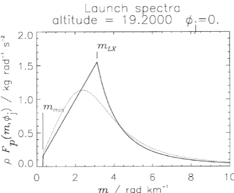
model, we choose the launch spectrum shown by the solid curve in Fig. 1. The dotted curve shows theω-integral ofˆ the pseudomomentum-flux launch spectrum in the full 3D power-spectral model. This last corresponds to the energy
1Momentum and pseudomomentum are distinct but related quantites that
appear in wave-mean interaction theory. Conservation of momentum is related to translational invariance of the physics, whereas conservation of pseudomomentum is related to translational invariance of the medium in which the waves propagate, as represented in linearized wave theory. The relevant components of their respective fluxes, i.e., the vertical fluxes of horizontal momentum and pseudomomentum, are equal, to sufficient ap-proximation, in our problem. However, the pseudomomentum flux can be equated to the vertical group velocity times the horizontal pseudomomen-tum density, which latter can be evaluated from linearized wave theory. For further discussion see WM96, above Eq. (13).
Fig. 1. Launch spectra of the verticalflux of horizontal pseudomomen-tum, integrated over the jth azimuthal sectorφ
j± 12φ. The sector sizeφ = 90◦ and j runs from 0 to 3. The solid curve is (4) and the dashed curve is (3). The total (one dimensional) pseudomomentum fluxρ(zL)Fp(1)(zL, φj)is identical for the two cases and is given by the (equal) areas under the curves. The characteristic vertical wavenumber
m∗=2π/(2 km)=3.142×10⁻³rad m−1, the crossover wavenumber mLX=m∗, and the small-mcutoffmmin=2π/(20 km)=3.142×10⁻⁴ rad m−1. Units formare rad km−1and for the 2D pseudomomentum fluxρ(zL)F(p2)(zL,m, φj)are kg (rad km−1)−1km−1s−2.
spectrum of Fritts and VanZandt (1993) apart from the in-troduction of a long wave cutoff at vertical wavenumber m=mmin.
More precisely, the dotted curve is theωˆ-integral of
ρ(zL)F(
which is the pseudomomentum-flux launch spectrum in the full 3D power-spectral model. Here ρ(zL) is the density at the launch altitudezL,β is an empirical constant, taken throughout this paper as 1.047×10⁻¹, while A
0, B0, and
0(=(2π)−1)are normalization constants for the vertical wavenumber spectrum, the intrinsic frequency spectrum and the azimuthal direction spectrum respectively and are
de-fined in WM96,m∗ is the “characteristic wavenumber”of the Fritts-VanZandt spectrum, NL is the value of the buoy-ancy frequency at the launch altitudez=zL, and the factors in the second and third lines of the equation come from tak-ing Coriolis and non-hydrostatic effects into account. The 2 sin(φ/2)factor is the result of integrating vectorally over the azimuthal sectorφj−φ/2< φ < φj+φ/2 centered on directionφj and of angular widthφ(see WM96). The notation ˆk0means the unit vectork0/|k0|. The subscript L
applied to any symbol indicates the value at the launch al-titude. The notational conventions used for the symbols for
fluxes with subscripts and superscripts are as follows. Tak-ing the above example,F(p3L), the bold font shows that this is a vector; the superscript(3)shows that the spectral space is 3D, subscriptpshows that this is aflux of pseudomomentum (subscript E would indicate aflux of wave energy); subscript L indicates, as before, that this is a launch altitudeflux.
When integrated over ωˆ, (2) yields the equation of the dotted curve, the CIRA summer value at 19.2 km altitude.
To allow efficient computation, the
pseudomomentum-flux launch spectrum in the 2D power-spectral model, the solid curve in Fig. 1, is defined by two power laws in dif-ferent ranges of m separated by a crossover wavenumber m(zL)= mLX, here taken somewhat arbitrarily to be equal because of the different spectral shapes.
In this paper, the powersformmin ≤ m <mLXwill be taken to bes=1 as suggested in Fritts and VanZandt (1993). In WM97, we found that this values =1 gives too large a contribution from ultra-long vertical wavelengths. In WM97 we tried adjustings(which, because it refers to the small-m end of the spectrum, is hardly constrained by gravity wave observations). However, gravity waves with vertical wave-lengths greater than 20 km are rarely if ever observed in the stratosphere. Therefore, somewhat arbitrarily, we keeps=1 as in WM96 but introduce a long-wave (small-m) cutoff at m=mmin. A reviewer has suggested that, when the model is used as a GCM parameterisation, the small-mcutoff should be set to the maximum wavenumber of vertically resolvable waves in the GCM. (This would presume that the model by itself correctly generates such waves.) Without the small-m cutoff, the model predicts turbulent energy dissipation rates
ε that appear to be unrealistically high, in comparison for instance with the rates observed by Lubken (1997).¨
require a more sophisticated explanation. For further discus-sion see WM96, also Hines (1991), Broutmanet al.(1997), and Eckermann (1997). The right hand part of the solid curve in Fig. 1, i.e., (4) in the rangemLX≤ m<∞, has just this m−3behavior, and is what we mean by the“quasi-saturated part”of the model spectrum.
2.2 Propagation
In the full 3D spectral description, each spectral compo-nent has a wavevectork=(k,l,−m), with zonal component k, meridional componentl and vertical component−m, to make m > 0 for upward propagating waves withω >ˆ 0 (i.e., sign conventions as in WM96). The horizontal projec-tion ofk, or the horizontal wavevector, isk0 =(k,l,0)=
k0(cosφj,sinφj,0), with magnitudek0=(k2+l2)1/2>0. Each such plane wave spectral component has an absolute frequency, or frequency relative to the ground, denoted by
ω0, which is invariant under propagation in a steady back-ground.
The intrinsic and absolute frequencies satisfy the Doppler-shift relation
ˆ
ω(z)=ω0−k0·U(z)=ω0−k0U(z), (5)
whereU(z)is the component of Uin the direction ofk0,
equivalently in theφjdirection. Because by definitionk0>0 and, for upward propagating waves,ω >ˆ 0, a positive vertical shear∂U/∂z >0 means thatωˆ will decrease in magnitude as altitudezincreases, corresponding to an approach toward critical-level conditions, promoting wavebreaking.
The vertical wavenumber m also varies with z under Doppler shifting; we use the abbreviations ωˆ1 = ˆω(z1), m1 = m(z1)andωˆ2 = ˆω(z2),m2 = m(z2)at altitudez1, z2, and similarly for the otherz-dependent quantities likeU and N. Substituting valuesU = U1 andU2 into (5), and subtracting to eliminateω0, we get
ˆ
ω1− ˆω2=k0U2−k0U1 (6)
for the Doppler shift in intrinsic frequencies betweenz1and z2. Substituting forωˆ1,ωˆ2using the dispersion relation (1) and dividing byk0, we obtain
Under the hydrostatic, non-rotating approximation, there-fore, the Doppler shifting of the vertical wavenumbermdoes not depend on the magnitude of the horizontal wavenumber k0.
This is crucial to the simplification used here and in Hines (1997a,b). It can be shown, and will be explained more fully in a forthcoming paper, that under such simplifications we can treat spectral propagation as a 2D problem in the same way as we treated the full 3D problem in WM96. The essence of the matter is that, under the approximation (1), theflow in (m,ωˆ) spectral space is such that elements do not tilt and stretch under Doppler shifting, as they do in the full evolution illustrated in Fig. 2 of WM96.
As in WM96, we can derive a spectral Jacobian to trans-form (2D) spectral elements in(m, φj)spectral space to the propagation-invariant spectral elements in(ω0, φj)spectral space. We can then use that Jacobian to calculate how the 2D
pseudomomentum fluxρ(z)F(2)
p (z,m, φj)varies from one altitude z to another under conservative propagation. We
find that
Having conservatively propagated the 2D spectrum from al-titude z1 up to altitudez2, we then impose as a ceiling the m−3 quasi-saturated behavior, that is, we require for allm
2
In other words, just as for the 3D case in WM96, we use the quasi-saturation spectrum (10) as a“chopping function”for
ρ(z)F(p2)(z,m, φj)at altitude zin the 2D model. We give the name“evolved spectrum”to thefinal 2D spectrum after propagation and chopping. The constantCLis the same as in (4), ensuring that the chopping function coincides with the right-hand part of the model launch spectrum—that is, coin-cides with (4) form≥mLX, i.e., to the right of the crossover wavenumbermLX. Although it can be argued that the con-stantCLin (10) should be taken to be a function of altitude, via its dependence on N(z), we choose for simplicity—as was done in WM96—to keepCLconstant, so that the altitude vari-ation ofρ(z)FpSis due only to the altitude variation,ρ(z), of the density for both the 2D and full 3D power-spectral models. In future work we plan to makeCL a function of altitude as a further step toward realism.
2.3 Computational procedure
The key to efficient computation is to assume that the evolving spectrum retains a piecewise structure as in (4), with smooth shapes except at crossover and cutoff wavenum-bersmX(z)andmmin(z). We may then take advantage of the power-law behavior of, respectively, the launch spectrum to the left of, and the chopping function to the right of, the crossover wavenumber.
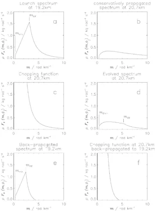
The actual computational procedure is now described for the case of positive shear, with reference to Fig. 2. Panels (a) and (b) respectively show the simplified launch spectrum (again forz =z1=zL =19.2 km) together with the result of conservatively propagating it up to z = z2 = 20.7 km through a positive wind incrementU2−U1 = +5 m s−1. Consistent with (7), the image of mLX = mX(zL) under Doppler shifting has gone off-scale to the right of panel (b), atm=11.2 rad km−1, whereas the image ofmminhas hardly shifted, by only 712% in this example, illustrating the extreme sensitivity of Doppler shifting tomvalues.
Fig. 2. Computational procedure for the ultra-simple spectral parameterisation for a positive background wind shear with incrementU2−U1= +5 m s−1; see text.
curve in panel (c), to chop the conservatively propagated spectrum shown in panel (b).
Panel (e) shows what will be called the artificially“ back-propagated spectrum” at 19.2 km or, for brevity, “ back-propagated spectrum”. By this we mean a spectrum that would result from running time backwards and conserva-tively propagating the evolved spectrum back down from 20.7 km to 19.2 km altitude. In other words, the back-propagated spectrum atz=zL(panel (e)) is just such as will propagate conservatively to produce the spectrum in panel (d) when time runs forwards. Note that the new crossover wavenumberm1Xin panel (e), which is the image of that in panel (d),m2X, under time-reversed Doppler shifting, lies to the left of the original crossover wavenumbermLX. That is, m1X<mLX. Finally, panel (f) shows the chopping function at 20.7 km (panel (c)) back-propagated to 19.2 km.
The aim is to compute the area under the curve in Fig. 2, panel (d), and other curves like it at other altitudesz. Note
first that this area is the same as the area in panel (e) because
back-propagation is by definition conservative. Second, the areas of the right and left hand parts—i.e., the parts to the right and left of the new crossover wavenumber—are sep-arately equal, because the relevant valuesm1Xandm2Xof the crossover wavenumber are connected via the Doppler re-lation (7). Third, the right hand area is easiest to compute analytically atz=z2because the chopping function (10) is a simple power law. By contrast, the left hand area is easiest to compute atz=z1(=zL), i.e., using panel (e) rather than panel (d), because it is the left half of panel (e) that has the simple power law behavior. The result is
ρ(z2)F(p1)(z2, φj)=
m1X
mmin
ρ(zL)F( 2)
pL(zL,m, φj)dm
+
∞
m2X
ρ(z2)F( 2)
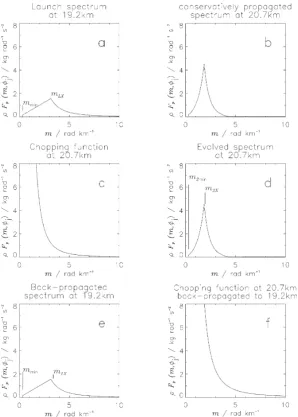
Fig. 3. Computational procedure for the ultra-simple spectral parameterisation for a negative background wind shear with incrementU2−U1= −5 m s−1; see text.
=
ρ(zL)CL msLX+1(s+1)
ms1X+1−msmin+1
+ρ(z2)CLm2LX 2
m−2X2
×2 sin(φ/2)kˆ0, (11)
where (cf. above (3)) the superscript(1)signals that all but one dimension of spectral space has been integrated out.
The crossover wavenumberm1Xis determined efficiently by using a Newton-Raphson method to locate the zero-crossing point of the back-propagated chopping function mi-nus the expression in the second line of (4). Thenm2X is obtained from (7).
The conditions typified by Fig. 2 assume thatmmin<m1X. Ifmmin≥m1Xthen the required modification is
ρ(z2)F(p1)(z2, φj)=
∞
m2 min
ρ(z2)F( 2)
pS(m, φj)dm
=
ρ(
z2)CLm2LX 2
m−2 min2
×2 sin(φ/2)kˆ0, (12)
wherem2 min=mmin(z2), defined by the appropriate Doppler shift, i.e., by substitutingm1=mmininto (7).
al-titudes, then the result will be a more complicated piecewise smooth curve, violating the assumptions used in deriving (11) and (12). Because of this, computingρ(z2)F(p1)(z2, φj) from (11) or (12) when the shear is negative can yield a re-sult that increases with altitude. This would correspond to waves that had previously broken being resurrected, which is clearly unphysical. We therefore insist, for all altitudesz, that
ρ(z)F(1)
p (z, φj)stay constant or decrease monotonically asz increases. Therefore, we accept the value ofρ(z)F(1)
p (z, φj) computed using (11) and (12) (withzreplacingz2) only if it is less than the values obtained for smallerz. For the case shown in Fig. 3 this amounts to substitutingm1X = mLX together with the correspondingm2X, obtained from(7), into (11). This is merely the simplest way of coping with the negative-shear case. We shall see that it may need some refinement; see Section 4.
2.4 Wave-induced forces per unit mass
As in WM96, we integrate-out the remaining spectral di-mension, the direction φin spectral space, to give, in dis-cretized form,
Here n is the number of discrete azimuthal sectors. The corresponding wave-induced force per unit mass isρ−1times the one-dimensional divergence ofρ(z)F(0)
The zonal and meridional components ofG(z)can now be calculated. They are readily calculated by substitutingF(1)
p (z, φj)for each sector into (14) in place ofF(p0)(z).
2.5 Turbulent dissipation
Observed turbulent dissipation rates due to breaking meso-spheric gravity waves (e.g., Lubken 1997) are an important¨
observational constraint on theoretical models. Turbulent dissipation can be estimated to afirst approximation as wave-energyflux convergences, i.e., neglecting work done by the turbulence against gravity (e.g., McIntyre, 1989). Comput-ing wave-energyfluxes for the ultra-simple spectral parame-terisation is carried out as follows. First the 2D wave-energy
fluxρ(z)FE(2)(z,m, φj)is written in terms of the 2D
pseudo-where the second line is obtained using the approximate dispersion relation (1). Then the 1D wave-energy flux
ρ(z)FE(1)(z, φj)for the jth sector is computed by integrat-ing over allm. For positive shear, the procedure is similar to that needed to obtain (11). Note that carrying out these integrations is not just a matter of scaling|ρ(z)F(1)
p (z, φj)|, because the m-dependences of ρ(z)FE(2)(z,m, φj) and
ρ(z)F(2)
p (z,m, φj)are different. However, under the hydro-static, non-rotating approximation the integrals are straight-forward to evaluate. Details are omitted for brevity.
For negative shear, we again use the simplest way of cop-ing. The relations (16) and (7), together with the condition
ρ(z)F(1) not necessarily a good approximation—it probably underes-timates the energyflux—but we defer attempts to improve it until the whole treatment of the negative-shear case is refined. On the above basis, the energy dissipation rate is given from the one-dimensional divergence of the wave-energyflux
ρ(z)FE(0)(z)=ρ(z)
n−1
j=0
FE(z, φj), (18)
together with a mean interaction term giving a wave-induced energy dissipation rate per unit mass
ε(z)= − 1 toε(z)from each sector are readily calculated by substituting F(1)
p (z, φj)into (19) in the place ofFp(0)(z)andF(
1)
E (z, φj)in the place ofFE(0)(z).
3.
Comparative Tests for the July, 40
◦N, CIRA
1986 Summer Case
The July, 40◦N, CIRA 1986 model atmosphere is shown in Fig. 4. We taken=4 in (13)–(15) corresponding to four azimuths, eastward, northward, westward, and southward (φj =0◦, 90◦, 180◦, and 270◦), and toφ =90◦. Spectra were launched from the zero of background zonal wind at an altitude of 19.2 km. The azimuthsφj =90◦and 270◦have no wind shear and so no Doppler shifts (k0normal toU). The
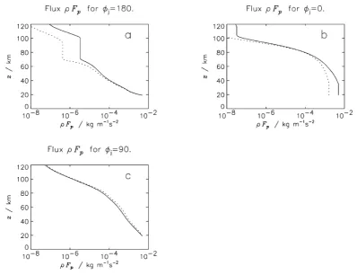
results forφj =90◦and 270◦will therefore be identical, so only theφj =90◦case will be shown. Two curves are shown in each panel of Figs. 5, 6, and 7. The solid curves are for the ultra-simple spectral parameterisation, and the dashed curves are for the full 3D power-spectral model. In each
figure, panel (a) shows theφj = 180◦ case, panel (b) the
φj =0◦ case, and panel (c) the 90≡270◦case. Panel (d), where present, shows information obtained by integrating over all azimuthal sectors.
Figure 5 shows the total pseudomomentumfluxρF(1)
p for
Fig. 4. July, 40◦N, CIRA 1986 summer profiles used in the comparison between the ultra-simple spectral parameterisation and the full 3D power-spectral model: (a) zonal mean zonal wind, (b) zonal mean buoyancy frequencyN(z), and (c) zonal mean temperatureT(z).
Fig. 5. Comparison of pseudomomentumfluxes for the ultra-simple model (solid curves) and the full model (dotted curves); see text.
one another. Here the ultra-simple model does remarkably well.
Next, consider the westward-propagating case shown in panel (a). Here waves are initially in positive background wind shear, and the two curves are seen to have a similar altitude dependence, although here the discrepancy between the models builds up to an order of magnitude difference in pseudomomentumflux at 70 km altitude. Between altitudes of 75 km and 95 km, where the background wind shear for these waves is strongly negative, there is hardly any wave
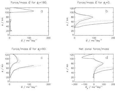
Fig. 6. Comparison of wave-induced forcesGper unit mass for the ultra-simple model (solid curves) and the full model (dotted curves); see text. The forces below about 70 km are plotted twice,first with the scale shown and second with a scale running from 0 to 20 m s−1in place of 0 to 200 m s−1.
causing the ultra-simple model to deposit some of the excess pseudomomentumflux. Both cases again show significant wave breaking but an order of magnitude moreflux is de-posited in the ultra-simple model than in the full model.
Finally, consider the eastward-propagating case shown in panel (b). It is here that we come up against the limitation of the ultra-simple model that derives from its inability to represent the back-reflection of waves Doppler shifted up to ωˆ = N. The full model, taking as it does the back-reflection into account, has cancelled about 70% of the up-ward pseudomomentumflux of the launch spectrum (dotted curve). The ultra-simple model has no means of doing this, as presently formulated, and so launches the full upwardflux (solid curve). Higher up, there is a remarkable cancellation of errors, in which the ultra-simple model breaks the waves too strongly, bringing theflux back toward agreement with the full model, but at the cost of producing a spurious wave-induced force especially in the important altitude range of the upper stratosphere (see concluding remarks).
Over the altitude range 19.2 km to 30 km, there is hardly any change in total pseudomomentumflux for both the ultra-simple model and the full model, the background wind shear being sufficiently negative to avoid wave breaking. Above 90 km, the two curves diverge again and, at the highest alti-tudes, there is more than an order of magnitude difference in pseudomomentumflux between the two cases.
Figure 6 shows the wave-induced force per unit massG for each azimuthal sector, together with the zonal component of wave induced forceGx. As the forces below about 70 km
can be very small they are plotted twice, the second set of curves scaled by a factor of 10. Considerfirst the northward-propagating, no wind shear, case shown in panel (c). The force G from the ultra-simple model is somewhat smaller than that from the full model over almost the entire altitude range, most obviously at the peak value around 90 km altitude where it is about 50% smaller. The falloff inGwith altitude above about 90 km is a consequence of choosingmmin = 2π/20 km. G starts to fall off from a higher altitude if a smaller value ofmminis chosen, and starts to fall off from a lower altitude if a larger value ofmminis chosen. In choosing an appropriatemmin, we are guided by observations such as those of Lubken (1997). More details are given below.¨
Fig. 7. Comparison of energy dissipation rates for the ultra-simple model (solid curves) and the full model (dotted curves); see text.
conspicuous.
The total wave-induced forceG, summed over azimuths
φj(which for this case is just the zonal component), is shown in panel (d). The peak values ofGare 94 m s−1day−1 east-ward at an altitude of 80 km for the ultra-simple model, (as compared with 81 m s−1day−1eastward at an altitude of 82 km for the full model), and 123 m s−1day−1westward at an altitude of 107 km for the ultra-simple model, (as compared with 7 m s−1day−1westward at an altitude of 107 km for the full model).
Recalling the original results of WM96, we note particu-larly the very significant effect of the choice ofmmin. The full model, withmmin=2π/20 km, now gives much smaller forces at the highest altitudes than it did in the cases studied in WM96, withmmin =0 ands =1, which gave a peakG value of 350 m s−1day−1westward at an altitude of 110 km. As will be seen below, our choice ofmmin can be justified to some extent by comparing energy dissipation rate curves from our two models with those of Lubken (1997).¨
Figure 7 shows the energy dissipation rate ε(z, φj) for each azimuthal sector, together with the energy dissipation rate ε(z) (the sum over all azimuths). Consider first the northward-propagating, no wind shear, case shown in panel (c). Above about 25 km, the curves differ by no more than a third of the energy dissipation rate for the ultra-simple model. The westward-propagating case in panel (a) has a sharp spike at about 100 km for the ultra-simple model case and not for the full model case. The presence of this fea-ture again shows the limitations of the simplifications we have made in going from the full model to the ultra-simple
model. The wave-energyflux (not shown) helps to explain this spike. At the top of the negative shear at about 100 km, the wave-energyflux for the ultra-simple model is over an order of magnitude larger than for the full model case. The change of sign of shear at 100 km altitude results in an immediate sharp drop in wave-energyflux over a single altitude increment and hence a sharp spike in the energy dis-sipation rate curve (approximately 40 times higher energy dissipation rate for the ultra-simple model than for the full model) that we see in Fig. 7, panel (a). In the eastward-propagating case shown in panel (b), the energy dissipation rate curves for the ultra-simple spectral parameterisation and the full 3D power-spectral model are very similar. Panel (d) showsε(z), the energy dissipation rate summed over all azimuthal directions. The obvious differences between the ultra-simple model and the full model are largely a conse-quence of the differences between the two models for the westward-propagating azimuth (panel (a)). If we look at the region below the sharp spike, the maximum value of the en-ergy dissipation rate curve (0·108 m2s−3=108 mW kg−1 at 80 km) is similar to that shown in Lubken (1997) (156¨
mW kg−1at 90 km) although its peak altitude is somewhat lower. Note, however that Lubken¨ ’s results are taken at 70◦N rather than 40◦N, and that a zonally averaged climatalogical average atmosphere may be a poor approximation to reality at these altitudes. We therefore now compare energy dissi-pation ratesε(z)for a range of values ofmminfor the July, 70◦N CIRA model atmosphere with Lubken¨ ’s results.
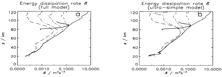
Fig. 8. Comparison of energy dissipation rates for various values ofmminwith the observational energy dissipation rates of L¨ubken (1997). Panel (a) shows the full model case and panel (b) the ultra-simple model case. (Bold full curves are observational data. Other curves are model data: full curves aremmin=2π/(100 km), dotted curves aremmin=2π/(50 km), dashed curves aremmin=2π/(20 km), dot-dashed curves aremmin=2π/(10 km), triple dot-dashed curves aremmin=2π/(5 km), and long dashed curves aremmin=2π/(2 km).)
data (Lubken, 1997) superimposed. Panel (a) of Fig. 8 shows¨
the full model case while panel (b) shows the ultra-simple model case. Our choice of 20 km formmin is seen to yield a comparable peak energy dissipation rate and altitude to Lubken¨ ’s result. Lubken¨ ’s observational energy dissipation rate peak is much more localised in altitude than is the case for either of our models. This may in part be because a zonally averaged climatological atmosphere may be a poor approximation to reality at these altitudes. Tests with more realistic profiles are planned.
4.
Concluding Remarks
The 2D power-spectral model at its current level of sim-plicity has three substantial shortcomings, which we hope to overcome by work in progress. Thefirst is the neglect of rota-tion in the dispersion relarota-tion (1), one of whose effects is the underestimation of wave-breaking as ωˆ is Doppler-shifted down toward f, in comparison with the wave breaking pre-dicted by the full 3D power-spectral model. The second shortcoming is the lack of back-reflection whenωˆ reaches N; see especially Fig. 5(b).
The third shortcoming is the underestimation of breaking after propagation in negative shear. The problem is due to the true spectral shape taking a very different form from the standard shape assumed in the 2D model. In particular, when a significant altitude range of negative shear is followed by an altitude range of positive shear, there is an underestimation of breaking in the negative-shear region and an overestimation in the positive-shear region. This is one cause of the sharp peak seen in the westward wave-induced force at the top of Fig. 6(a), and in dissipation rate at the top of Fig. 7(a).
The discrepancies between 2D and 3D models are too large for comfort. There is also the problem that (for both mod-els) the force in the summertime upper stratosphere has the wrong sign. A westward force appears critical to the upper branch of the poleward summertime stratospheric circula-tion (Rosenlof, 1996), and hence to the transport of water vapor from there up into the mesosphere, and hence to the formation of noctilucent and polar mesospheric clouds.
Acknowledgments. This work received support from the Natural Environment Research Council through Grant GR3/1163, through
the U.K. Universities’Global Atmospheric Modelling Project, and through the IGWOC project which is supported by the EC Environ-ment and Climate Research Programme (Contract: ENV4-CT97-0486, Climate and Natural Hazards).
References
Broutman, D., C. Macaskill, M. E. McIntyre, and J. W. Rottman, On Doppler-spreading models of internal waves,Geophys. Res. Lett.,24, 2813–2816, 1997.
Dewan, E. M. and R. E. Good, Saturation and the“universal”spectrum for vertical profiles of horizontal scalar winds in the atmosphere,J. Geophys. Res.,91, 2742–2748, 1986.
Eckermann, S. D., Influence of wave propagation on the Doppler spreading of atmospheric gravity waves,J. Atmos. Sci.,54, 2554–2573, 1997. Fritts, D. C. and W. Lu, Spectral estimates of gravity wave energy and
momentumfluxes II: Parameterisation of wave forcing and variability,J. Atmos. Sci.,50, 3695–3713, 1993.
Fritts, D. C. and T. E. VanZandt, Spectral estimates of gravity wave en-ergy and momentumfluxes. Part I: Energy dissipation, acceleration, and constraints,J. Atmos. Sci.,50, 3685–3694, 1993.
Hines, C. O., The saturation of gravity waves in the middle atmosphere. Part I: Critique of linear-instability theory,J. Atmos. Sci.,48, 1348–1359, 1991.
Hines, C. O., Doppler-spread parameterization of gravity-wave momentum deposition in the middle atmosphere. 1. Basic formulation,J. Atmos. Sol.-Terr. Phys.,59(4), 371–386, 1997a.
Hines, C. O., Doppler-spread parameterization of gravity-wave momentum deposition in the middle atmosphere. 2. Broad and quasi monochromatic spectra, and implementation,J. Atmos. Sol.-Terr. Phys.,59(4), 387–400, 1997b.
Lubken, F.-J., Seasonal variation of turbulent energy dissipation rates at¨ high latitudes as determined by in situ measurements of neutral density fluctuations,J. Geophys. Res.,102(D12), 13441–13456, 1997. McIntyre, M. E., On the dynamics and transport near the polar mesopause
in summer,J. Geophys. Res.,94, 14617–14628, 1989.
Rosenlof, K., Summer hemisphere differences in temperature and transport in the lower stratosphere,J. Geophys. Res.,101, 19129–19136, 1996. Smith, S. A., D. C. Fritts, and T. E. VanZandt, Evidence of a saturated
spectrum of atmospheric gravity waves,J. Atmos. Sci.,44, 1404–1410, 1987.
Warner, C. D. and M. E. McIntyre, On the propagation and dissipation of gravity wave spectra through a realistic middle atmosphere,J. Atmos. Sci.,53, 3213–3235, 1996.
Warner, C. D. and M. E. McIntyre, Gravity wave spectral models and the shapes of gravity wave spectra at low vertical wavenumbers, in Grav-ity Wave Processes: Their Parameterization in Global Climate Models, edited by Kevin Hamilton, pp. 217–226, Springer-Verlag, Heidelberg, 1997.