Sequential Parameter Estimation of Time-Varying
Non-Gaussian Autoregressive Processes
Petar M. Djuri´c
Department of Electrical and Computer Engineering, State University of New York at Stony Brook, Stony Brook, NY 11794, USA Email: [email protected]
Jayesh H. Kotecha
Department of Electrical and Computer Engineering, University of Wisconsin, Madison, WI 53706, USA Email: [email protected]
Fabien Esteve
ENSEEIHT/T´eSA 2, rue Charles Camichel, BP 7122, 31071 Toulouse Cedex 7, France Email: [email protected]
Etienne Perret
ENSEEIHT/T´eSA 2, rue Charles Camichel, BP 7122, 31071 Toulouse Cedex 7, France Email: [email protected]
Received 1 August 2001 and in revised form 14 March 2002
Parameter estimation of time-varying non-Gaussian autoregressive processes can be a highly nonlinear problem. The problem gets even more difficult if the functional form of the time variation of the process parameters is unknown. In this paper, we address parameter estimation of such processes by particle filtering, where posterior densities are approximated by sets of samples (particles) and particle weights. These sets are updated as new measurements become available using the principle of sequential importance sampling. From the samples and their weights we can compute a wide variety of estimates of the unknowns. In absence of exact modeling of the time variation of the process parameters, we exploit the concept of forgetting factors so that recent measurements affect current estimates more than older measurements. We investigate the performance of the proposed approach on autoregressive processes whose parameters change abruptly at unknown instants and with driving noises, which are Gaussian mixtures or Laplacian processes.
Keywords and phrases:particle filtering, sequential importance sampling, forgetting factors, Gaussian mixtures.
1. INTRODUCTION
In on-line signal processing, a typical objective is to process incoming data sequentially in time and extract information from them. Applications vary and include system identifi-cation [1], equalization [2, 3], echo cancelation [4], blind source separation [5], beamforming [6, 7], blind deconvolu-tion [8], time-varying spectrum estimadeconvolu-tion [6], adaptive de-tection [9], and digital enhancement of speech and audio sig-nals [10]. These applications find practical use in communi-cations, radar, sonar, geophysical explorations, astrophysics, biomedical signal processing, and financial time series anal-ysis.
The task of on-line signal processing usually amounts to estimation of unknowns and tracking them as they change with time. A widely adopted approach to addressing this
Another approach to tracking time-varying signals is par-ticle filtering [19]. The underlying approximation imple-mented by particle filters is the representation of densities by samples (particles) and their associated weights. In
par-ticular, if x(m) andw(m), m = 1,2, . . . , M, are the samples
and their weights, respectively, one approximation of p(x) is
given by
whereδ(·) is Dirac’s delta function. The approximation of
the densities by particles can be implemented sequentially, where as soon as the next observation becomes available, the set of particles and their weights are updated using the Bayes rule. Some of the basics of this procedure are reviewed in this paper. The recent interest in particle filters within the sig-nal processing community has been initiated in [14], where a special type of particle filters are used for target tracking. Since the particle filtering methods are computationally in-tensive, the continued advancement of computer technology in the past few years has played a critical role in sustaining this interest. An important feature of particle filtering is that it can be implemented in parallel, which allows for major speedups in various applications.
One advantage of particle filters over other methods is that they can be applied to almost any type of problem where signal variations are present. This includes models with high nonlinearities and with noises that are not necessarily Gaus-sian. In all the work on particle filtering presented in the wide literature, it is assumed that the applied model is com-posed of a state equation and an observation equation, where the state equation describes the dynamics of the tracked sig-nal (or parameters). Thus, the use of particle filters requires knowledge of the functional form of the signal (parameter) variations. In this paper, we make the assumption that this
model isnotavailable, that is, we have no information about
the dynamics of the unknowns. In absence of a state equa-tion, we propose to use a random walk model for describ-ing the time variation of the signal (or parameters). We show that the random walk model implies forgetting of old mea-surements [20, 21]. In other words, it assigns more weight to more recent observations than to older measurements.
In this paper, we address the problem of tracking the parameters of a non-Gaussian autoregressive (AR) process whose parameters vary with time. The usefulness of the mod-eling of time series by autoregressions is well documented in the wide literature [22, 23]. Most of the reported work, how-ever, deals with stationary Gaussian AR processes, and right-fully so because many random processes can be modeled suc-cessfully with them. In some cases, however, the Gaussian AR models are inappropriate, as for instance, for processes that contain spikes, that is, samples with large values. Such signals are common in underwater acoustic, communications, oil exploration measurements, and seismology. In all of them, the processes can still be modeled as autoregressions, but with non-Gaussian driving processes, for example, Gaussian mixture or Laplacian processes. Another deviation from the
standard AR model is the time-varying AR model where the parameters vary with time [21, 24, 25, 26, 27, 28, 29].
The estimation of the AR parameters of non-Gaussian
AR models is a difficult task. Parameter estimation of such
models has rarely been reported, primarily due to the lack of tractable approaches for dealing with them. In [30], a max-imum likelihood estimator is presented and its performance is compared to the Cramer-Rao bound. The conditional like-lihood function is maximized by a Newton-Raphson search algorithm. This method obviously cannot be used in the set-ting of interest in this paper. In a more recent publication, [31], the driving noises of the AR model are Gaussian mix-tures, and the applied estimation method is based on a gen-eralized version of the expectation-maximization principle.
When the AR parameters change with time, the problem
of their estimation becomes even more difficult. In this
pa-per, the objective is to address this problem, and the applied methodology is based on particle filtering. In [32, 33], parti-cle filters are also applied to estimation of time-varying AR models, but the driving noises there are Gaussian processes.
The paper is organized as follows. In Section 2, we for-mulate the problem. In Section 3, we provide a brief re-view of particle filtering. An important contribution of the paper is in Section 4, where we propose particle fil-ters with forgetting factors. The proposed method is ap-plied to time-varying non-Gaussian autoregressive processes in Section 5. In Section 6, we present simulation examples, and in Section 7, we conclude the paper with some final re-marks.
2. PROBLEM FORMULATION
Observed data yt,t=1,2, . . ., represent a time-varying AR
process of orderK that is excited by a non-Gaussian noise.
The data are modeled by
yt=
K
k=1
atkyt−k+vt, (2)
where vt is the driving noise of the process, andatk, k =
1,2, . . . , K, are the parameters of the process at timet. The values of the AR parameters are unknown, but the model
order of the AR process, K, is assumed known. The
driv-ing noise process is independently and identically distributed (i.i.d.) and non-Gaussian, and is modeled as either a Gaus-sian mixture with two mixands, that is,
vt∼(1−)ᏺ0, σ12
whereα >0. In this paper, we assume that the noise
param-eters,,σ12,andσ22of the Gaussian mixture process andαof
the Laplacian noise are known. The objective is to track the
3. PARTICLE FILTERS
Many time-varying signals of interest can be described by the following set of equations:
xt= ftxt−1, ut
, yt=htxt, vt, (5)
wheret∈Nis a discrete-time index,xt∈Ris an unobserved
signal att,yt∈Ris an observation, andut ∈Randvt ∈R
are noise samples. The mapping ft:R×R→Ris referred to
as a signal transition function, andht:R×R→R, as a
mea-surement function. The analytic forms of the two functions are assumed known. Generalization of (5) to include vector observations and signals as well as multivariable functions is straightforward.
There are three different classes of signal processing
prob-lems related to the model described by (5):
(1) filtering: for allt, estimatextbased ony1:t,
tive is to carry out the estimation of the unknownsrecursively
in time.
A key expression for recursive implementation of the es-timation is the update equation of the posterior density of x1:t= {x1, x2, . . . , xt}, which is given by
Under the standard assumptions thatutandvtrepresent
ad-ditive noise and are i.i.d. according to Gaussian distributions
and that the functions ft(·) andht(·) are linear inxt−1andxt,
respectively, the filtering, prediction, and smoothing prob-lems are optimally resolved by the Kalman filter [12]. When the optimal solutions cannot be obtained analytically, we re-sort to various approximations of the posterior distributions [12, 13].
The set of methods known as particle filtering methods are based on a very interesting paradigm. The basic idea is to represent the distribution of interest as a collection of
sam-ples (particles) from that distribution. We drawMparticles,
ᐄt={x(tm)}Mm=1, from a so-called importance sampling
distri-butionπ(x1:t |y1:t). Subsequently, the particles are weighted
aswt(m) = p(x(1:mt)|y1:t)/(π(x(1:mt)|y1:t)). Ifᐃt = {wt(m)}Mm=1,
then the setsᐄtandᐃtcan be used to approximate the
pos-terior distributionp(xt|y1:t) as in (1), or
It can be shown that the above estimate converges in
distri-bution to the true posterior asM → ∞[34]. More
impor-tantly, the estimate of Ep(g(xt)), where Ep(g(·)) is the
ex-pected value of the random variableg(xt) with respect to the
posterior distributionp(xt|y1:t), can be written as
Thus, the particles and their weights allow for easy compu-tation of minimum mean square error (MMSE) estimates. Other estimates are also easy to obtain.
Due to the Markovian nature of the state equation, we can develop a sequential procedure called sequential
impor-tance sampling (SIS), which generates samples from p(x1:t |
y1:t) sequentially [14, 35]. As new data become available, the
particles are propagated by exploiting (6). In this sequential-updating mechanism, the importance function has the form
π(xt |x1:t−1, y1:t), which allows for easy computation of the
particle weights. The ideal importance function minimizes the conditional variance of the weights and is given by [36]
πxt|x1:t−1, y1:t
The SIS algorithm can be summarized as follows.
(1) At timet=0, we generateMparticles fromπ(x0) and
and weights for timetfrom steps 3, 4, and 5.
(3) Form=1, . . . , M, drawx(tm)∼π(xt|x(1:mt−)1, y1:t).
(5) Normalize the weights using
wt(m)=
An important problem that occurs in sequential Monte Carlo methods is that of sample degeneration. As the re-cursions proceed, the importance weights of all but a few of the trajectories become insignificant [35]. The degener-acy implies that the performance of the particle filter will be very poor. To combat the problem of degeneracy, resampling
is used. Resampling effectively throws away the trajectories
manner. Let{x(tm), wt(m)}Mm=1be the weights and particles that
are being resampled. Then
(1) form=1, . . . , M, generate a number j ∈ {1, . . . , M}
represents the new sets of weights and particles.
Improved resampling in terms of speed can be imple-mented using the so-called systematic resampling scheme [37] or stratified resampling [38].
Much of the activity in particle filtering in the sixties and seventies was in the field of automatic control. With the advancement of computer technology in the eighties and nineties, the work on particle filters intensified and many new contributions appeared in journal and conference pa-pers. A good source of recent advances and many relevant references is [19].
4. PARTICLE FILTERS WITH FORGETTING FACTORS In many practical situations, the function that describes the
time variation of the signals ft(·) is unknown. It is unclear
then how to apply particle filters, especially keeping in mind that a critical density function needed for implementing the recursion in (6) is missing. Note that the form of the density
p(xt|xt−1) depends directly on ft(·). In [20], we argue that
this is possible and can be done in somewhat similar way as with methods known as recursive least squares (RLS) with discounted measurements [22]. Recall that the idea there is to minimize a criterion of the form
εt=
etis an error that is minimized and given by
et=yt−dt (14)
withdtbeing a desired signal. The tracking of the unknowns
is possible without knowledge of the parametric function of
their trajectories because withλ <1, the more recent
mea-surements have larger weights than the meamea-surements taken further in the past. In fact, we apply implicitly a window to
our data that allows more recent data to affect current
esti-mates of the unknowns more than old data.
In the case of particle filters, we can replicate this phi-losophy by introducing a state equation that will enforce the “aging” of data. Perhaps the simplest way of doing it is to have a random walk model in the state equation, that is,
xt=xt−1+ut, (15)
where ut is a zero mean random sample that comes from
a known distribution. Now, if the particlesxt(−m1) with their
weightswt(−m1)approximatep(xt−1|y1:t−1), with (15) the
dis-tribution ofxt will be wider due to the convolution of the
densities ofxt−1andut. It turns out that this implies
forget-ting of old data, where the forgetforget-ting depends on the
param-eters ofp(ut). For example, the larger the variance ofut, the
faster is the forgetting of old data [20]. Additional theory on the subject can be found in [21] and the references therein. In the next section we present the details of implementing this approach to the type of AR processes of interest in this paper.
5. ESTIMATION OF TIME-VARYING NON-GAUSSIAN AUTOREGRESSIVE PROCESSES BY PARTICLE FILTERS
The observation equation of an AR(K) process can be
writ-ten as
yt=aT
tyt+vt, (16)
whereaT
t ≡ (at1, . . . , atK) andyt ≡ (yt−1, . . . , yt−K)T. Since
the dynamic behavior of at is unknown, as suggested in
Section 4, we model it with a random walk, that is,
at=at−1+ut, (17)
whereutis a known noise process from which we can draw
samples easily. It is reasonable to choose the noise process as a
zero mean Gaussian with covariance matrixΣut. The
covari-ance matrixΣut is then set to vary with time by depending
on the covariance matrixΣat−1. For example, for the AR(1)
whereλis the forgetting factor. From (17), we get
σ2
Similarly, forK >1, we can choose
Σut =Σdiag
whereΣdiagis a diagonal matrix whose diagonal elements are
equal to the diagonal elements ofΣat−1.
Now, the problem is cast in the form of a dynamic state space model, and a particle filtering algorithm for
sequen-tial estimation of at can readily be applied as discussed in
Section 4. An important component of the algorithm is the
importance function,π(at|a1:t−1, y1:t), which is used to
gen-erate the particlesa(tm).
The algorithm can be outlined as follows.
(1) Initialize{a(0m)}Mm=1by obtaining samples from a prior
distributionp(a0) and let ¯w0(m) =1 form=1, . . . , M. Then
for each time step repeat steps 2, 3, 4, 5, and 6.
(2) Compute the covariance matrix ofatand obtain the
(3) Fori =1, . . . , M, obtain samplesa(tm) from the
im-If the noise is Laplacian, the update is done by
¯
wt(m)=wt(−m1)e−α|yt−a
(m)T
t yt|. (23)
(5) Normalize the weights according to
wt(m)=
(6) Resample occasionally or at every time instant from
{a(tm), wt(m)}Mm=1to obtain particles of equal weights.
6. SIMULATION RESULTS
We present, next, results of experiments that show the perfor-mance of the proposed approach. In all our simulations we
usep(at|at−1) as the importance function. First, we show a
simple example that emphasizes the central ideas in this
pa-per. We estimated recursively the coefficient of an AR(1)
pro-cess with non-Gaussian driving noise. The data were gener-ated according to
experiment, and that its value was fixed to 0.99. A random
walk was used as the process equation to impose forgetting of measurements, that is,
at=at−1+ut, (26)
whereut was zero mean Gaussian with varianceσ2
ut chosen
according to (19) with forgetting factor λ = 0.9999. The
number of particles wasM = 2000. For comparison
pur-poses, we applied a recursive least squares (RLS) algorithm
whose forgetting factor was alsoλ = 0.9999.1One
particu-lar representative simulation is shown in Figure 1. Note that
awas tracked more accurately using the particle filter
algo-rithm. Similar observations were made in most simulations.
1It should be noted that the RLS algorithm is not based on any proba-bilistic assumption, and that it is computationally much less intensive than the particle filtering algorithm.
0 100 200 300 400 500 600 700 800 900 1000
Forgetting factor=0.9999, number of particles=2000
Figure 1: Estimation of an autoregressive parameterausing the RLS and particle filtering methods. The parameterawas fixed and was equal to 0.99.
1 2 3 4 5 6 7
Number of particles: 50, 100, 200, 500, 1000, 2000, 4000 0
Figure 2: Mean square error of the particle filter and the RLS method averaged over 20 realizations. The driving noise was a Gaus-sian mixture.
With data generated by this model, we compared the performances of the particle filter and the RLS for various number of particles. The methods were compared by their MSEs averaged over 20 realizations. The results are shown
in Figure 2. It is interesting to observe that forM =50 and
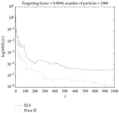
0 100 200 300 400 500 600 700 800 900 1000
Forgetting factor=0.9999, number of particles=2000
Figure3: Evolution of the log(MSEi(t)) of the particle filter and the RLS method.
RLS filter. As expected, as the number of particles increased, the performance of the particle filter improved considerably. In Figure 3, we present the evolution of the instantaneous mean square errors as a function of time of the particle filter-ing and the RLS methods. The instantaneous mean square errors were obtained from 20 realizations, and
MSEi(t)=
where ˆaj,tis the estimate ofatin the jth realization. For the
particle filter we usedM =2000 particles, andλ= 0.9999.
Clearly, the particle filter performed better. It is not surpris-ing that the largest errors occur at the beginnsurpris-ing, since there the methods have little prior knowledge of the true value of
the parametera.
In the next experiment, the noise was Laplacian. There,
the parameterαwas varied and had values 10, 2, and 1. In
Figure 4, we present the MSEs of the particle filter and the RLS estimate averaged over 20 realizations. The particle filter
clearly outperformed the RLS for all values ofα.
The results of the first experiment with time-varying AR
parameters are shown in Figure 5. There,a was attributed
a piecewise changing behavior where it jumped from 0.99
to 0.95 at the time instantt = 1001, and the driving noise
was a mixture Gaussian as in the first experiment. The
for-getting factor λwas 0.95. Note that both the RLS and the
particle filter follow the jump. However, the particle filter tracks it with higher accuracy and lower variation. Note also that the variation in the estimates in this experiment is much higher since the chosen forgetting factor was much smaller.
Statistical results of this experiment are shown in Figure 6. The figure shows the MSEs of the particle filter and
1 2 3
Laplacian distribution parameters: 10, 2, and 1 0
×10−4 Forgetting factor=0.9999, number of particles=1000
Particle filter RLS
Figure 4: Mean square error of the particle filter and the RLS method averaged over 20 realizations. The driving noise was Lapla-cian.
0 200 400 600 800 1000 1200 1400 1600 1800 2000 t
Forgetting factor=0.95, number of particles=2000
Figure5: Tracking performance of the piecewise constant AR pa-rameteratwith a jump from 0.99 to 0.95 att=1001.
the RLS method averaged over 20 realizations as functions of time. The particle filter outperformed the RLS significantly.
The experiment was repeated for a jump ofafrom 0.99
to−0.99 att=1001. Two different values of forgetting
fac-tors were used,λ = 0.99 andλ =0.95, and the number of
particles was kept atM=2000.In Figures 7 and 8, we
plot-ted MSE(t) obtained from 20 realizations. It is obvious from
the figures that the performance of the particle filter was not
0 200 400 600 800 1000 1200 1400 1600 1800 2000
Forgetting factor=0.95, number of particles=2000
Figure6: Evolution of the log(MSEi(t)) of the particle filter and the RLS method. The driving noise was mixture Gaussian.
0 200 400 600 800 1000 1200 1400 1600 1800 2000 t
forgetting factor=0.95, number of particles=2000
Figure7: Evolution of the log(MSEi(t)) of the particle filter and the RLS method. The forgetting parameter wasλ=0.95, and the number of particles wasM=2000.
is the importance function of the particle filter. The prior importance function does not expect a change at that time because it does not use observations for generating particles.
As a result, the particles att=1001 are generated around the
values ofa(1000m), which are all faraway from the actual value
ofa. Moreover, it took the particle filter more than 700
sam-ples to “regroup,” and that is a consequence of the relatively high value of the forgetting factor. When this value was
de-creased toλ=0.9, the recovery of the particle filter was much
shorter (see Figure 8). Note that the price for improvement
0 200 400 600 800 1000 1200 1400 1600 1800 2000 t
forgetting factor=0.9, number of particles=2000
Figure8: Evolution of the log(MSE(t)) of the particle filter and the RLS method. The forgetting parameter wasλ=0.9, and the number of particles wasM=2000.
was a larger MSE during the periods of time whenawas
con-stant. We can enhance the performance of the particle filter by choosing an importance function, which explores the
pa-rameter space ofabetter.
In another experiment we generated data with higher or-der AR models. In particular, the data were obtained by
yt= −0.7348yt−1−1.8820yt−2−0.7057−yt−3
The driving noise was a Gaussian mixture with the same parameters as in the first experiment. The tracking of the parameters by the particle filter and the RLS method from one realization is shown in Figure 9. The number of particles
wasM=2000 and the forgetting factorλ=0.9. In Figure 10,
we display the MSE errors of the two methods as functions of time.
Another statistical comparison between the two meth-ods is shown in Figure 11. There, we see the average MSEs of the methods presented separately for each parameter and
for various forgetting factors. The number of particlesM =
8000. The particle filter performed better fora2t,a3t, anda4t,
but worse fora1t. A reason for the inferior performance of
the particle filter in tracking a1t is perhaps due to the big
change of values ofa1t, which requires smaller forgetting
fac-tor than the one used. More importantly, with better
im-portance function the tracking performance ofa1t can also
0 500 1000 1500
Autoregressive parametera1
0 500 1000 1500
t
Autoregressive parametera2
0 500 1000 1500
t
Autoregressive parametera3
0 500 1000 1500
t
Autoregressive parametera4
Figure9: Tracking of the AR parameters, where the models change att=501 andt=1001.
0 500 1000 1500
t
Autoregressive parametera1
0 500 1000 1500
t
Autoregressive parametera2
0 500 1000 1500
t
Autoregressive parametera3
0 500 1000 1500
t
Autoregressive parametera4
1 2 3 Forgetting factor: 0.86, 0.88, 0.9 0
Autoregressive parametera1
1 2 3
Forgetting factor: 0.86, 0.88, 0.9 0
Autoregressive parametera2
1 2 3
Forgetting factor: 0.86, 0.88, 0.9 0
Autoregressive parametera3
1 2 3
Forgetting factor: 0.86, 0.88, 0.9 0
Autoregressive parametera4
Figure11: Mean square error of each of the AR parameters produced by the particle filter and the RLS method averaged over 20 realizations. The driving noise was mixture Gaussian.
the region of the new values of the parameters, and thereby would produce a more accurate approximation of their pos-terior density.
7. CONCLUSIONS
We have presented a method for tracking the parameters of a time-varying AR process which is driven by a non-Gaussian noise. The function that models the variation of the model parameters is unknown. The estimation is carried out by par-ticle filters, which produce samples and weights that approx-imate required densities. The state equation that models the parameter changes with time is a random walk model, which implies the discounting of old measurements. In the simu-lations, the parameters of the process are piecewise constant where the instants of their changes are unknown. The piece-wise model is not by any means a restriction imposed by the method, but was used for convenience. Simulation results were presented. The requirement of knowing the noise pa-rameters that drive the AR process can readily be removed.
REFERENCES
[1] L. Ljung and T. S¨oderstr¨om, Theory and Practice of Recursive Identification, MIT Press, Cambridge, Mass, USA, 1983. [2] R. W. Lucky, “Automatic equalization for digital
communica-tions,” Bell System Technical Journal, vol. 44, no. 4, pp. 547– 588, 1965.
[3] J. G. Proakis, Digital Communications, McGraw-Hill, New York, NY, USA, 3rd edition, 1995.
[4] K. Murano, S. Unagami, and F. Amano, “Echo cancellation and applications,” IEEE Communications Magazine, vol. 28, pp. 49–55, January 1990.
[5] S. Haykin, Ed., Unsupervised Adaptive Filtering: Blind Source Separation, vol. I ofAdaptive and Learning Systems for Signal Processing , Communications, and Control, Wiley Interscience, New York, NY, USA, 2000.
[6] S. Haykin, Adaptive Filter Theory, Prentice-Hall, Upper Saddle River, NJ, USA, 3rd edition, 1996.
[7] P. W. Howells, “Explorations in fixed and adaptive resolution at GE and SURC,”IEEE Transactions on AP, vol. 24, pp. 575– 584, 1975.
[8] S. Haykin, Ed., Unsupervised Adaptive Filtering: Blind Decon-volution, vol. II ofAdaptive and Learning Systems for Signal Processing , Communications, and Control, Wiley, New York, NY, USA, 2000.
[9] B. Widrow and S. D. Stearns, Adaptive Signal Processing, Prentice-Hall, Englewood Cliffs, NJ, USA, 1985.
[10] S. Godsill and P. Rayner, Digital Audio Restoration—A Sta-tistical Model Based Approach, Springer, New York, NY, USA, 1998.
[12] B. D. Anderson and J. B. Moore,Optimal Filtering, Prentice-Hall, Englewood Cliffs, NJ, USA, 1979.
[13] A. H. Jazwinski,Stochastic Processes and Filtering Theory, Aca-demic Press, New York, NY, USA, 1970.
[14] N. J. Gordon, D. J. Salmond, and A. F. M. Smith, “Novel ap-proach to nonlinear/non-Gaussian Bayesian state estimation,”
IEE Proceedings Part F: Radar and Signal Processing, vol. 140, no. 2, pp. 107–113, 1993.
[15] D. L. Alspach and H. W. Sorenson, “Nonlinear Bayesian es-timation using Gaussian sum approximation,”IEEE Transac-tions on Automatic Control, vol. 17, no. 4, pp. 439–448, 1972. [16] S. Fr¨uhwirth-Schnatter, “Data augmentation and dynamic
linear models,” Journal of Time Series Analysis, vol. 15, no. 2, pp. 183–202, 1994.
[17] G. Kitagawa, “Non-Gaussian state-space modeling of nonsta-tionary time series,”Journal of the American Statistical Associ-ation, vol. 82, no. 400, pp. 1032–1063, 1987.
[18] S. Julier, J. Uhlmann, and H. F. Durrant-Whyte, “A new method for the nonlinear transformation and covariances in filters and estimator,”IEEE Transactions on Automatic Control, vol. 45, no. 3, pp. 477–482, 2000.
[19] A. Doucet, N. de Freitas, and N. Gordon, Eds., Sequential Monte Carlo Methods in Practice, Springer, New York, NY, USA, 2001.
[20] P. M. Djuri´c, J. Kotecha, J.-Y. Tourneret, and S. Lesage, “Adap-tive signal processing by particle filters and discounting of old measurements,” inProc. IEEE Int. Conf. Acoustics, Speech, Sig-nal Processing, Salt Lake City, Utah, USA, 2001.
[21] M. West,Bayesian Forecasting and Dynamic Models, Springer-Verlag, New York, NY, USA, 1997.
[22] M. H. Hayes,Statistical Digital Signal Processing and Modeling, Wiley, New York, NY, USA, 1996.
[23] S. M. Kay, Modern Spectral Estimation, Prentice-Hall, Engle-wood Cliffs, NJ, USA, 1988.
[24] R. Charbonnier, M. Barlaud, G. Alengrin, and J. Menez, “Re-sults on AR modeling of nonstationary signals,” Signal Pro-cessing, vol. 12, no. 2, pp. 143–151, 1987.
[25] K. B. Eom, “Time-varying autoregressive modeling of HRR radar signatures,” IEEE Trans. on Aerospace and Electronics Systems, vol. 36, no. 3, pp. 974–988, 1999.
[26] Y. Grenier, “Time-dependent ARMA modeling of nonstation-ary signals,”IEEE Trans. Acoustics, Speech, and Signal Process-ing, vol. 31, no. 4, pp. 899–911, 1983.
[27] M. G. Hall, A. V. Oppenheim, and A. D. Wilsky, “Time vary-ing parametric modelvary-ing of speech,” Signal Processing, vol. 5, pp. 276–285, 1983.
[28] L. A. Liporace, “Linear estimation of nonstationary signals,”
J. Acoust. Soc. Amer., vol. 58, no. 6, pp. 1288–1295, 1975. [29] T. S. Rao, “The fitting of nonstationary time series models
with time-dependent parameters,” J. Roy. Statist. Soc. Ser. B, vol. 32, no. 2, pp. 312–322, 1970.
[30] D. Sengupta and S. Kay, “Efficient estimation of param-eters for non-Gaussian autoregressive processes,” IEEE Trans. Acoustics, Speech, and Signal Processing, vol. 37, no. 6, pp. 785–794, 1989.
[31] S. M. Verbout, J. M. Ooi, J. T. Ludwig, and A. V. Oppenheim, “Parameter estimation for autoregressive Gaussian-mixture processes: The EMAX algorithm,”IEEE Trans. Signal Process-ing, vol. 46, no. 10, pp. 2744–2756, 1998.
[32] A. Doucet, S. J. Godsill, and M. West, “Monte Carlo filter-ing and smoothfilter-ing with application to time-varyfilter-ing spectral estimation,” inProc. IEEE Int. Conf. Acoustics, Speech, Signal Processing, vol. II, pp. 701–704, Istanbul, Turkey, 2000.
[33] S. Godsill and T. Clapp, “Improvement strategies for Monte Carlo particle filters,” inSequential Monte Carlo Methods in Practice, A. Doucet, N. de Freitas, and N. Gordon, Eds., Springer, 2001.
[34] J. Geweke, “Bayesian inference in econometrics models using Monte Carlo integration,” Econometrica, vol. 57, pp. 1317– 1339, 1989.
[35] J. S. Liu and R. Chen, “Sequential Monte Carlo methods for dynamic systems,”Journal of the American Stastistical Associ-ation, vol. 93, no. 443, pp. 1032–1044, 1998.
[36] A. Doucet, S. J. Godsill, and C. Andrieu, “On sequential Monte Carlo sampling methods for Bayesian filtering,” Statis-tics and Computing, vol. 10, no. 3, pp. 197–208, 2000. [37] J. Carpenter, P. Clifford, and P. Fearnhead, “An improved
par-ticle filter for non-linear problems,” IEE Proceedings Part F: Radar, Sonar and Navigation, vol. 146, no. 1, pp. 2–7, 1999. [38] E. R. Beadle and P. M. Djuri´c, “A fast weighted Bayesian
boot-strap filter for nonlinear model state estimation,”IEEE Trans. on Aerospace and Electronics Systems, vol. 33, no. 1, pp. 338– 342, 1997.
Petar M. Djuri´creceived his B.S. and M.S. degrees in electrical engineering from the University of Belgrade, Yugoslavia, in 1981 and 1986, respectively, and his Ph.D. degree in electrical engineering from the Univer-sity of Rhode Island in 1990. From 1981 to 1986 he was Research Associate with the Institute of Nuclear Sciences, Vinˇca, Bel-grade, Yugoslavia. Since 1990 he has been with State University of New York at Stony
Brook, where he is Professor in the Department of Electrical and Computer Engineering. He works in the area of statistical signal processing, and his primary interests are in the theory of model-ing, detection, estimation, and time series analysis and its applica-tion to a wide variety of disciplines, including telecommunicaapplica-tions, biomedicine, and power engineering. Prof. Djuri´c has served on numerous Technical Committees for the IEEE and SPIE, and has been invited to lecture at universities in the US and overseas. He was Associate Editor of the IEEE Transactions on Signal Process-ing, and currently he is the Treasurer of the IEEE Signal Processing Conference Board. He is also Vice-Chair of the IEEE Signal Process-ing Society Committee on Signal ProcessProcess-ing—Theory and Meth-ods, and a Member of the American Statistical Association and the International Society for Bayesian Analysis.
Jayesh H. Kotechareceived his B.E. in elec-tronics and telecommunications from the College of Engineering, Pune, India in 1995, and M.S. and Ph.D. degrees in electrical engineering from the State University of New York at Stony Brook in 1996 and 2001, respectively. Since January 2002, he has been with the University of Wisconsin at Madison as a postdoctoral researcher. Dr. Kotecha’s research interests are chiefly in the
Fabien Esteve received the Engineer de-gree in electrical engineering and signal processing in 2002 from ´Ecole Nationale Sup´erieure d’ ´Electronique, d’ ´Electrotech-nique, d’Informatique, d’Hydraulique et des T´el´ecommunications (ENSEEIHT), Toulouse, France.
Etienne Perret was born in Albertville, France in 1979. He received his Engineer degree in electrical engineering and signal processing and M.S. in microwave and optical telecommunications from ´Ecole Nationale Sup´erieure d’ ´Electronique, d’ ´Electrotechnique, d’Informatique, d’Hy-draulique et des T´el´ecommunications (ENSEEIHT), Toulouse, France. He is cur-rently working toward his Ph.D. degree at