http://siba-ese.unisalento.it/index.php/ejasa/index
e-ISSN: 2070-5948
DOI: 10.1285/i20705948v10n1p50
Bayesian estimation of the Rayleigh distribution under different loss function
By Boudjerda et al.
Published: 26 April 2017
This work is copyrighted by Universit`a del Salento, and is licensed un-der aCreative Commons Attribuzione - Non commerciale - Non opere derivate 3.0 Italia License.
For more information see:
DOI: 10.1285/i20705948v10n1p50
Bayesian estimation of the Rayleigh
distribution under different loss function
K. Boudjerda
a, A. Chadli
∗a, A. Merradji
a, and H. Fellag
baProbability Statistics laboratory; University Badji Mokhtar BP12, 23000 Annaba, Algeria, bMouloud Mammeri University; Tizi-Ouzou, Algeria
Published: 26 April 2017
In a Rayleigh distribution, We are interested in the estimation of the pa-rameter and some reliability characteristics, as the reliability and the failure rate functions. We used the Bayesian approach under different loss function (squared loss and Linex loss) with a type II censored data. The prior law of the parameter is non-informative prior then a natural conjugated prior. The estimators ofσ, S(t) andh(t) are obtained with the exact analytic ex-pression, the posterior risks are calculated in each case. A simulation study was carried out as well as real data analysis. A comparison between the different estimators from there posterior risks leads us to conclude that the best estimator is obtained under the Linex loss function.
keywords: Rayleigh distribution, Bayesian estimation, Posterior risk, Linex loss function.
1 Introduction
Lord Rayleigh (1880) introduced the Rayleigh distribution in connection with a prob-lem in the field of acoustics. Since then, extensive work has taken place related to this distribution in different areas of science and technology. Its has some nice relations with some of well known distribution like Weibull, Chi-square or extreme distributions. The origin and other aspects of this distribution can be found in Siddiqui.
The Rayleigh distribution is a special case of the two parameter Weibull distribution and a suitable model for life testing studies. Polovko, (1968), Dyer and Whisenand,(1973),
∗
Corresponding author: [email protected]
c
Universit`a del Salento ISSN: 2070-5948
demonstrated the importance of this distribution in electro vacuum devices and commu-nication engineering.
The probability density function (pdf), the reliability function and the failure rate func-tion, respectively are given by:
f(x, σ) = x σ2exp(− x2 2σ2), x >0, σ >0 (1) S(x, σ) =exp(− x 2 2σ2) (2) and h(x, σ) = x σ2 (3)
Whereσ >0 is the parameter. An important characteristics of the Rayleigh distribution is that its failure rate is an increasing linear function of time. This means that when the failure times are distributed according to the Rayleigh law, an intense aging of the equipment takes place. Then as time increases the reliability function decreases at a much higher rate than in the case of exponential distribution.
Several authors have studied the Rayleigh distribution, Howlader and Hossain (1995) studied the problem of the estimation of the parameter and the reliability function with censored data and squared loss function. Dyer and Whisenand, (1973), provided the best linear unbiased estimator of σ based on complete sample, censored sample and selected order statistics. Bayesian estimation and prediction problems for the Rayleigh distribution based on doubly censored sample have been considered by Balakrishnan, (1989), Fernandez, (2000), Raqab and Madi, (2011). Bayesian estimation problems for the Rayleigh distribution based on progressively censored sample have been considered by Kim and Han, (2009), Raqab and Madi,(2011), and Dey and Dey, (2014).
In this paper, we study the Bayesian estimator of the parameter, reliability function and the failure rate function under squared loss function and asymmetric loss function in presence of censored type II sample with non-informative prior density and conjugate prior.
Notation
b
σM L: Maximum likelihood estimator of the parameterσ.
b
σSV: Bayesian estimator of the parameter σ under the squared loss function with a
vague prior.
R(σbSV): Posterior risk ofσbSV. b
σLV: Bayesian estimator of the parameter σ under the Linex loss function with a
vague prior.
R(σbLV): Posterior risk ofσbLV.
SM L(t): Maximum likelihood estimator of the reliability function.
SSV(t): Bayesian estimator of the reliability function under the squared loss function
with a vague prior.
R(SM L(t)): Posterior risk of SM L(t).
SLV(t): Bayesian estimator of the reliability function under the Linex loss function
with a vague prior.
R(SLV(t)): Posterior risk of SLV(t).
hM L(t): Maximum likelihood estimator of the failure rate function.
hSV(t): Bayesian estimator of the failure rate function under the squared loss function
with a vague prior.
R(hSV(t)): Posterior risk of hSV(t).
hLV(t): The Bayesian estimator of the failure rate function under the Linex loss
function with a vague prior.
R(hLV(t)): Posterior risk ofhLV(t).
b
σCS: Bayesian estimator of the parameter σ under the squared loss function with a
natural conjugated prior.
R(σbCS): Posterior risk ofbσCS. b
σCL: Bayesian estimator of the parameterσunder the Linex loss function with natural
conjugated prior.
R(σbCL): Posterior risk ofσbCL.
SCS(t): Bayesian estimator of the reliability function under squared loss function with
natural conjugated prior.
R(SCS(t)): Posterior risk ofSCS(t).
SCL(t): Bayesian estimator of the reliability function under the Linex loss function
with natural conjugated prior.
R(SCL(t)): Posterior risk ofSCL(t).
hCS(t): Bayesian estimator of the failure rate function under Linex loss function with
natural conjugated prior.
R(hCS(t)): Posterior risk of hCS(t).
hCL(t): Bayesian estimator of the failure rate function under the Linex loss function
with natural conjugated prior.
2 Bayesian estimation with non-informative prior
Let (X(1), X(2), ..., X(r), ..., X(n)) a sample of sizencensored inX(r)The likelihood writes: L(x|σ)∝ 1 σ2rexp(− Tr 2σ2) or Tr= r X i=1 x2i + (n−r)x2r
In the Bayesian context, when we have few or no information of the parameter, we use vague priors. The most popular is due to Jeffreys et al. defined as follows:
π1(σ) =|I1(σ)| 1 2 =| −E∂ 2lnf ∂σ2 | ∝ 1 σ The posterior density is then:
π1(σ|x) = L(x|σ)π1(σ) R∞ 0 L(x|σ)π1(σ)dσ = (Tr) r Γ(r) 1 2r−1σ −2r−1exp(− Tr 2σ2)
Or xis the vector of observations.
2.1 Loss functions
2.1.1 Squared loss function
Let θbthe estimator of θ, the squared loss function defined by L1(θ,θb) = (θ−θb)2 is
proposed by Legendre (1805) and Gauss (1810), it is widely used in literature. The Bayesien estimator ofθ is then the posterior mean, letθbB=E(θ|x).
2.1.2 Linex loss function
The Linex (Linear Exponential) loss function is dominantly and widely used because it is a natural extension of squared loss function. It was originally introduced by Varian Varian, (1975), and got a lot of popularity due to Zellner Zellner, (1986).
The mathematical form of Linex loss function may simply be expressed by: L(∆)∝ea∆−a∆−1 , a6= 0.
Where ∆ = (θb−θ), θbis an estimate of θ.
Consider the following convex loss function:
L(∆)∝ea∆−a∆−1, a6= 0 (4)
The signe of a and its absolute magnitude represent the direction and the degree of asymmetry. For a → 0, we find the squared loss function. Varian (1975) considered the loss function in (4) for ∆1 = θb−θ; the function L(∆1) is called the Linex loss
function. LetEp(L(∆1)) the posterior expectation of L(∆1), the Bayesian estimator of θunder this loss function is denotedθbLB it corresponds to the value ofθbthat minimizes
Ep(L(∆1)). (Ep is the mean with respect to the posterior density).
Ep(L(∆1)) =expa(θb)Ep(exp(−aθ)) +aEp(θ)−aθb−1 (5)
We derive the above expression with respect toθband we equal to zero
∂Ep(L(∆1)) ∂θb
=a(exp(aθb))Ep(exp(−aθ))−a= 0
The solution of this equation is:
b
θLB =−
1
aln(Ep(e
−aθ))
Consider the loss functionL(∆2); or ∆2 = (bθθ)2−1; this loss function has been used by
several authors whose Zellner (2006) and (2009). We minimize the posterior expectation Ep(L(∆2)): Ep(L(∆2)) =Ep[exp(( b θ θ) 2−1)−a((bθ θ) 2−1)−1] =exp(−a)Ep(exp( b θ θ) 2)−a(θb θ) 2−1
We derive Ep(L(∆2)) with respect to θband we equal to zero, we obtain the Bayesian
estimator θbLB of θ under the loss functionL(∆2)
∂Ep(L(∆2)) ∂bθ = 2a(exp(−a))Ep( b θ θ2exp(a( b θ θ) 2))−2aE p( b θ θ2) = 0 b
θLB is then the solution of the equation
Ep[ 1 θ2exp(a( b θLB θ2 ))] =exp(a)Ep( 1 θ2) (6)
2.2 Estimation of the parameter σ
The maximum likelihood estimator denoted bσM L is obtained by solving the equation
∂lnL(x,σ) ∂σ = 0; then: b σM L= r Tr 2r (7)
With respect to the squared loss function, and with a vague prior onσ; the estimator of σ denoted bσSW is obtained with calculate its expectation with respect to the posterior
density: b σSV = Z ∞ 0 σπ(σ|x)dσ= (Tr) r Γ(r) 1 2r−1 Z ∞ 0 σ−2rexp(− Tr 2σ2)dσ= Γ(r−12) Γ(r) ( Tr 2 ) 1 2 (8)
The posterior risk of the parameterσ is given by R(bσV Q) = ( Tr 2 )( Γ(r−1) Γ(r) − Γ2(r−1 2) Γ2(r) ). (9)
With respect to squared loss function L(∆2) and the vague prior, the estimator of σ
denoted bσLV is the solution of equation given in (5) or:
Ep[b σLV σ2 exp(a( b σ2LV σ2 ))] = (Tr)r Γ(r) b σLV 2r−1 Z ∞ 0 1 σ2r+3exp(− 1 2σ2(Tr−2aσb 2 LV))dσ and exp(a)Ep(b σLV σ2 ) = (Tr)r Γ(r) b σLV 2r−1 Z ∞ 0 1 σ2r+3exp(− 1 2σ2(T r) )dσ After some algebraic manipulations, we obtain:
b σLV = [ Tr 2a(1−exp(− a r+ 1))] 1 2 (10)
the posterior risk of the parameter σ under the Linex loss function is given by:
R(bσLV) =a(σbSV −σbLV). (11)
2.3 Estimation of the reliability function
for obtain the estimator SM L(t) of the reliability S(t), we replace σ with bσM L in the
expression ofS(t), then
SM L(t) =exp(−
rt2 Tr
) (12)
The Bayesien estimator of S(t) with respect to the squared loss function and the vague prior isSSV(t) SSV(t) = Z ∞ 0 S(t)π1(σ|x)dσ= ( Tr Tr+t2 )r (13)
The posterior risk of the reliability function under the squared loss function is given by: R(SSV(t)) = ( Tr Tr+ 2t2 )r−( Tr Tr+t2 )2r (14)
The Bayesian estimator ofS(t) with respect to the Linex loss function is denotedSLV(t),
for calculate, we make the following change of variable: S(t) =exp(−2tσ22) =γ ⇒ σ =
(−2lnγt2 )12; we write the posterior density according toγ
π1(γ|x) = (Tr)r Γ(r) 1 2r−1 1 2(− t2 2lnγ) 1 2( t 2 2γ(lnγ)2)(− t2 2lnγ) −r−1 2(γ) Tr t2 = (Tr t2) r 1 Γ(r)(γ) Tr t2−1(−lnγ)r−1; 0≤γ ≤1
We used the loss function L(∆1), The Bayesian estimatorγLV of γ, is
γLV =−
1
alnEp(exp(−aγ)) =− 1 aln[( Tr t2) r 1 Γ(r) Z ∞ 0 exp(−aγ)(γ)Trt2−1(−lnγ)r−1dγ] =−1 aln[ k X j=0 (−a)j j! (1 +j t2 Tr )−r] (15)
The last result is obtained by using a development of (exp(−aγ)) to order kin a neigh-borhood of zero and making the change variable u = (−lnγ) to the calculation of this integral.
The posterior risk of the reliability function under the Linex loss function is given by R(SLV(t)) =a(SSV(t)−SLV(t)) (16)
2.4 Estimation of the failure rate function
The maximum likelihood estimator of h(t) denotedhM L(t) is obtained when we replace
σ with bσM L in the expression of h(t), then:
hM L(t) = 2r
t Tr
(17) With respect to the squared loss function and a vague prior ofσ, the Bayesian estimator of h(t) denoted hSV(t) is: hSV(t) = Z ∞ 0 h(t)π1(σ|x)dσ= (Tr)r Γ(r) t 2r−1 Z ∞ 0 σ−2r−3exp(− Tr 2σ2)dσ hSV(t) = 2r t Tr (18) The posterior risk of the failure rate function under the squared loss function is:
R(hSV(t)) = 4t2Γ(r+ 2) Γ(r) (Tr) −2−(2r)2 t2 (Tr)2 (19) Remark : The estimator ofh(t) obtained by maximum likelihood estimation and with the Bayesian approach with the non-informative prior and squared loss function are identical.
The asymmetric loss functionsL(∆1) andL(∆2) are not appropriate for a simple analytic
form of a Bayesian estimatorh(t); that is why, we define ∆ = (θ
b
θ −1) and we replace in
the loss function given by (4), then we take the posterior expectation, we drift and we equal to zero to find the value of θdenoted θbLV which minimizes
Ep(L(∆)) =Ep(exp(a( θ b θ −1)))−aEp( θ b θ −1)−1
∂Ep(L(∆)) ∂θb =exp(−a)Ep(−a θ b θ2exp( θ b θ)) +aEp( θ b θ 2 ) = 0
The Bayesian estimator θbLV with respect to the loss function L(∆) is then the solution
of the equation: exp(−a)Ep(θexp(a( θ b θV L ))) =Ep(θ) (20) We place h(t) = θ, let σt2 =θ⇒σ = (tθ) 1
2, we write the posterior density according to θ: π1(θ|x) = (Tr)r Γ(r) 1 2r−1( t θ) −r−1 2exp(−Tr 2tθ) 1 2( t θ) −1 2( t θ2) = (Tr 2t) r 1 Γ(r)θ r−1exp(−Tr 2tθ); θ≥0.
We remark that the posterior law of θis a gamma G(r,Tr
2t).
We solve the equation (20), orθbLV is the estimator of the failure rateh(t) and we denoted
hLV(t) exp(−a)(Tr 2t) r 1 [Tr 2t − a hV L(t)] r+1 = 2t Tr hLV(t) =a 2t Tr [1−exp(− a r+ 1)] −1 (21)
The posterior risk of the failure rate function under the Linex loss function is given by: R(hLV(t)) =a(hLV(t)−hSV(t)) (22)
3 Bayesian estimation with a natural conjugated prior
The naturel conjugated prior is defined as:π2(σ)∝
1
σα+1exp(− β
2σ2); α, β >0 (23)
The posterior law is then:
π2(σ|x) = (Tr+β)r+ α 2 2r+α2−1Γ(r+α 2) 1 σ2r+α+1exp(− 1 2σ2(Tr+β)) Remark
3.1 Estimation of the parameter σ
Always with respect to the squared loss function but with a natural conjugated prior of σ; the estimator of σ denoted bσCS is obtained when we calculate its expectation with
respect to the posterior density:
b σCS= Z ∞ 0 σπ2(σ|x)dx= r Tr+β 2 Γ(r+α2 −1 2) Γ(r+α2) (24) The posterior risk of the parameterσ is given by the following formula:
R(σbCS) = Tr+β 2 ( Γ(r+ α2 −1) Γ(r+ α2) − Γ2(r−α2 −12) Γ2(r−α 2) ) (25)
The Bayesian estimator ofσ with respect toL(∆2) and the natural conjugated prior of σ,σ denoted σbCL is the solution of the equation:
Ep[b σCL σ2 exp(a( b σ2CL σ2 ))] = 2 r+α2 b σCL[ Γ(r+α2 + 1) (Tr+β−2abσ 2 CL) r+α2+1] exp(a)Ep(b σCL σ2 ) =bσCLe a Γ(r+α2 + 1) (Tr+β)r+ α 2+1 b σCL= [ Tr+β 2a (1−exp(− a r+ α2 + 1))] 1 2 (26)
The posterior risk of the parameterσ under the Linex loss function is given by:
R(σbCL) =a(σbCS−bσCL) (27)
3.2 Estimation of the reliability function
The Bayesian estimator ofS(t) with respect to the squared loss function and the natural conjugated prior is SCS(t) SCS(t) = Z ∞ 0 S(t)π2(σ|x)dσ= ( Tr+β Tr+β+t2 )r+α2 SCS(t) = ( Tr+β Tr+β+t2 )r+α2 (28)
The posterior risk of the reliability function under the squared loss function is given by: R(SCS(t)) = ( Tr+β Tr+β+ 2t2 )r+α2 −( Tr+β Tr+β+t2 )2r+α (29) with a natural conjugated prior, the Bayesian estimator with respect to the Linex loss function is denoted SCL(t), for calculate, we use the following variable change: S(t) =
exp(− t2
2σ2) =γ ⇒σ = (− t 2 2lnγ)
1
2; we write the posterior density according toγ. γCQ =
−1
= −1 a ln[ (Tr+β)r+ α 2 Γ(r+α2) 1 (t2)r+α2 Z ∞ 0 exp(−aγ)(γ)Trt+2β−1(−lnγ)r+α2−1dγ] =−1 aln[ k X 0 (−a)j j! (1 + jt2 Tr+β )(−r−α2)] (30)
The posterior risk of the reliability function under the Linex loss function is given by R(SCL(t)) =a(SCS(t)−SCL(t)) (31)
3.3 Estimation of the failure rate function
with respect to the squared loss function, the Bayesian estimator is given by: hCS(t) = Z h(t, σ)π2(σ|t)dt= 2(r+α2) Tr+β t (32)
The posterior risk of the failure rate function is given by: R(hCS(t)) = ( t 2) 2Γ(r+ α 2 + 2) Γ(r+α2) (Tr+β) −2−h CS(t)2 (33)
Under the Linex loss function, the Bayesian estimator of the failure rate function is given by the following formula:
hCL(t) =a 2t Tr+β [1−exp(− a r+α2 + 1)] −1 (34)
The posterior risk of the failure rate function under the Linex loss function is:
R(hCL(t)) =a(hCS(t)−hCL(t)) (35)
4 Simulations
In this section, we propose to study the performance of the Bayesian estimators of the reliability function and the parameter under some various loss functions with respect to the MLE. An exhaustive Monte Carlo comparative study is performed using the loss functions given in the previous sections.
Firstly, we take (α, β) = (1,2) and we generate the natural conjugated prior ofσ, given by expression (23) and we deduce the values of σ (we obtain that σ = Γ(12) = 1.7724 the initial value ofσ)
We generateN = 10000 sample size ofnof the rayleigh distribution of the parameter σ(we used the Inversion method) witch have the cumulative distribution function (CDF) given by: F(x, σ) = 1−S(x, σ) = 1−exp(−x2
2σ2) , we take tree values ofn(n= 20,30,50)
and two values ofr (r= 10,15) for get increasing censured rate.
We calculate the maximum likelihood estimators of σ, S(t) and h(t) (denoted ML), then, we calculate the Bayesian estimators under the squared loss function (denoted S)
and under the Linex loss function for three values of a(LI1 (a=−0.5), LI2 (a=−1), LI3 (a= 1)).
For each estimator, we calculate mean squared error (MSE) given by the expression below, φconsideredσ,S(t), and h(t), φbhis estimator respectively
M SE(φ) = 1 N N X i=1 (φ−φb)2.
The values of MSE are given between brackets in the first cologne of the table 1. Tn the case of Bayesian estimators, we calculate the posterior risk (denoted PR) (the expression analytic of PR are given by (9), (11), (14), (16), (19), (22), (25), (27), (29), (31), (33), (35)).
In the following tables, we present the results of the Monte-Carlo study, in the first table the prior law is a vague prior, but in the second table we consider the natural conjugated prior.
Table 1: Bayesian estimators of the Rayleigh distribution with a vague prior
(n,r) φ ML(MSE) S(PR) LI1(PR) LI2(PR) LI3(PR)
(20,10) σ 1.7494(0.0005) 1.8187(0.0021) 1.6872(0.0072) 1.7084(0.0041) 1.6272(0.0210) S(t) 0.9058(0.0048) 0.9063(0.0049) 0.8841(0.0023) 0.8402(0.0017) 0.6825(0.0235) h(t) 0.2651(0.0006) 0.2651(0.0006) 0.2850(0.0021) 0.2791(0.0016) 0.3067(0.0046) (30,10) σ 1.7513(0.0044) 1.8106(0.0023) 1.6990(0.0069) 1.7081(0.0041) 1.6310(0.0199) S(t) 0.9059(0.0048) 0.9063(0.0049) 0.8841(0.0023) 0.8403(0.0002) 0.6827(0.0253) h(t) 0.2652(0.0007) 0.2652(0.0007) 0.2859(0.0021) 0.2788(0.0016) 0.3048(0.0043) (50,10) σ 1.7478(0.0006) 1.8170(0.0019) 1.6856(0.0075) 1.7090(0.0040) 1.6332(0.0193) S(t) 0.9059(0.0006) 0.9065(0.0049) 0.8845(0.0023) 0.8398(1.46e-05) 0.6824(0.0235) h(t) 0.2656(0.0007) 0.2656(0.0007) 0.2856(0.0021) 0.2780(0.0015) 0.3048(0.0043) (20,15) σ 1.7557(0.0002) 1.8012(0.0008) 1.7157(0.0032) 1.7285(0.0019) 1.6760(0.0092) S(t) 0.9086(0.0052) 0.9089(0.0053) 0.8867(0.0025) 0.8105(10-05) 0.6838(0.0231) h(t) 0.2565(0.0003) 0.2565(0.0003) 0.2684(0.0008) 0.2645(0.0006) 0.2812(0.0018) (30,15) σ 1.7625(9e-05) 1.8082(0.0012) 1.7200(0.0027) 1.7238(0.0018) 1.6710(0.0102) S(t) 0.9033(0.0053) 0.9096(0.0054) 0.8871(0.0026) 0.8426(4e-05) 0.6837(0.0231) h(t) 0.2543(0.0002) 0.2543(0.0002) 0.2671(0.0008) 0.2642(0.0006) 0.2830(0.0019) (50,15) σ 1.7551(0.0002) 1.8006(0.0007) 1.7119(0.0036) 1.7299(0.0018) 1.67421(0.0096) S(t) 0.9085(0.0003) 0.9088(0.0052) 0.8864(0.0025) 0.8427(4e-05) 0.6838(0.0237) h(t) 0.2566(0.0003) 0.2566(0.0003) 0.2693(0.0009) 0.2451(0.0006) 0.2818(0.0018)
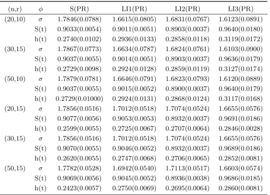
Table 2:Bayesian estimators Rayleigh with a natural conjugated prior
(n,r) φ S(PR) LI1(PR) LI2(PR) LI3(PR)
(20,10) σ 1.7846(0.0788) 1.6615(0.0805) 1.6831(0.0767) 1.6123(0.0891) S(t) 0.9033(0.0054) 0.9011(0.0051) 0.8903(0.0037) 0.9640(0.0180) h(t) 0.2740(0.0102) 0.2936(0.0133) 0.2858(0.0118) 0.3119(0.0172) (30,15) σ 1.7867(0.0773) 1.6634(0.0787) 1.6824(0.0761) 1.6103(0.0900) S(t) 0.9037(0.0055) 0.9014(0.0051) 0.8903(0.0037) 0.9636(0.0179) h(t) 0.2729(0.0098) 0.2924(0.0128) 0.2859(0.0119) 0.3127(0.0174) (50,10) σ 1.7879(0.0781) 1.6646(0.0791) 1.6823(0.0793) 1.6120(0.0889) S(t) 0.9037(0.0055) 0.9015(0.0052) 0.8900(0.0037) 0.9640(0.0179) h(t) 0.2729(0.01000) 0.2924(0.0131) 0.2868(0.0124) 0.3117(0.0168) (20,15) σ 1.7856(0.0516) 1.7012(0.0518) 1.7074(0.0524) 1.6655(0.0576) S(t) 0.9077(0.0056) 0.9053(0.0053) 0.8932(0.0037) 0.9691(0.0186) h(t) 0.2599(0.0055) 0.2725(0.0067) 0.2707(0.0064) 0.2846(0.0028) (30,15) σ 1.7856(0.0516) 1.7012(0.0518) 1.7074(0.0524) 1.6655(0.0576) S(t) 0.9070(0.0055) 0.9046(0.0052) 0.8932(0.0037) 0.9689(0.0186) h(t) 0.2620(0.0055) 0.2747(0.0068) 0.2706(0.0065) 0.2852(0.0081) (50,15) σ 1.7782(0.0528) 1.6942(0.0540) 1.7113(0.0517) 1.6603(0.0574) S(t) 0.9069(0.0056) 0.9045(0.0052) 0.8936(0.0038) 0.9686(0.0185) h(t) 0.2423(0.0057) 0.2750(0.0069) 0.2695(0.0064) 0.2860(0.0081)
After this simulation study, we conclude that the estimator of the parameter has a minimum risk when we used the squared loss function and the best estimator of the reliability function is obtained with Linex loss function (a=−1).
5 Data Analysis
We apply the proposed methods to areal data set presented in Lawless. The data arose in test on the endurance of deep-groove bearings and are originally discussed by Lieblein and Zelen. They are the number of revolutions to failure for each of n = 23 bearings in the life test. Raqab and Madi indicated that a one parameter Rayleigh distribution acceptable for these data. Here we consider n = 23 deep-groove ball bearing failure times. The 23 failure times are:
0.1788, 0.2892, 0.3300, 0.4152, 0.4212, 0.4560, 0.4848, 0.5184, 0.5196, 0.5412, 0.5556, 0.6780, 0.6864, 0.6864, 0.6888, 0.8412, 0.9312, 0.9864, 1.0512, 1.0584, 1.2792, 1.2804, 1.7304.
The maximum likelihood estimator of the parameter σ is equal to bσM L = 0.9175
For different values oft= 0.25,0.5,0.75,1, we obtain the maximum likelihood estimators of the reliability function that areSM L(t) = 0.9635, 0.8620, 0.7160, 0.5521
The maximum likelihood estimator of the failure rate function for different values of t are: bhM L(t) = 0.2969, 0.5939, 0.8908, 1.1878
The Bayesian estimators of the parameters σ, the reliability function and the failure rate function with a wave prior, then with a natural conjugated prior are given in the following tables:
Table 3:Bayesian estimators of the Rayleigh distribution with a vague prior and real data
t φ S(PR) LI1(PR) LI2(PR) LI3(PR)
0.25 σ 0.9451(0.0187) 0.9001(0.0449) 0.8921(0.0264) 0.8686(0.0765) h(t) 0.5939(0.0271) 0.6170(0.0231) 0.6282(0.0171) 0.6170(0.0231) 0.75 S(t) 0.7190(0.0042) 0.7144(0.0045) 0.7189(2.14*10−5) 0.7378(0.0188) h(t) 0.8908(0.0610) 0.9255(0.0346) 0.9423(0.0257) 0.9940(0.1031) 1 S(t) 0.5594(0.0078) 0.5603(0.0008) 0.5609(0.0007) 0.5628(0.0033) h(t) 1.1878(0.1085) 1.2340(0.0462) 1.2564(0.0343) 1.3275(0.1375)
Table 4:Bayesian estimators of Rayleigh distribution with a natural conju-gated prior and real data
t φ S(PR) LI1(PR) LI2(PR) LI3(PR)
0.25 σ 0.9473(0.0181) 0.6075(0.3397) 0.6051(0.1710) 0.5980(0.3493) S(t) 0.9638(0.0654) 0.9065(0.0581) 0.9176(0.0231) 0.9852(0.0214) h(t) 0.2949(0.0064) 0.3059(0.0110) 0.3113(0.0082) 0.3277(0.0328) 0.5 S(t) 0.8635(0.1843) 0.7124(0.1511) 0.7173(0.0731) 0.7124(0.1511) h(t) 0.5898(0.0257) 0.6117(0.0220) 0.6226(0.0164) 0.6118(0.0220) 0.75 S(t) 0.7205(0.2371) 0.4772(0.2432) 0.4776(0.1214) 0.4783(0.2421) h(t) 0.8847(0.0579) 0.9178(0.0331) 0.9339(0.0246) 0.9833(0.0986) 1 S(t) 0.5614(0.2015) 0.2731(0.2882) 0.2723(0.1445) 0.2697(0.2916) h(t) 1.1796(0.1030) 1.2237(0.0441) 1.2452(0.0328) 1.3111(0.1315)
6 Conclusion
In this paper, we studied the problem of Bayesian parameter estimation, reliability func-tion and failure rate funcfunc-tion in Rayleigh model with typeII censored data. The interest of this work is that the analytical expression of these different estimators and their pos-teriori risks could be explicitly given under each loss function (Linex and quadratic).
Data analysis and simulation lead to the conclusion that the estimators h(t) and R(t) are better under a Linex loss function fort relatively large.
Acknowledgements
The authors are grateful for the comments and suggestions by the referee and the Editor. Their comments and suggestions greatly improved the article.
References
Balakrishnan, N. (1989). Approximate mle of the scale parameter of the rayleigh distri-bution with censoring. IEEE Transactions on Reliability, 38(3):355–357.
Dey, S. and Dey, T. (2014). Statistical inference for the rayleigh distribution under pro-gressively type-ii censoring with binomial removal. Applied Mathematical Modelling, 38(3):974–982.
Dyer, D. D. and Whisenand, C. W. (1973). Best linear unbiased estimator of the pa-rameter of the rayleigh distribution-part i: Small sample theory for censored order statistics. IEEE Transactions on Reliability, 22(1):27–34.
Fernandez, A. J. (2000). Bayesian inference from type ii doubly censored rayleigh data.
Statistics & probability letters, 48(4):393–399.
Howlader, H. and Hossain, A. (1995). On bayesian estimation and prediction from rayleigh based on type ii censored data. Communications in Statistics-Theory and Methods, 24(9):2251–2259.
Jeffreys, A. J., Wilson, V., Thein, S. L., et al. (1985). Hypervariableminisatellite regions in human dna. Nature, 314(6006):67–73.
Kim, C. and Han, K. (2009). Estimation of the scale parameter of the rayleigh distri-bution under general progressive censoring. Journal of the Korean Statistical Society, 38(3):239–246.
Lawless, J. F. (2011). Statistical models and methods for lifetime data. John Wiley & Sons.
Lieblein, J. and Zelen, M. (1956). Statistical investigation of the fatigue life of deep-groove ball bearings. Journal of Research of the National Bureau of Standards, 57(5):273–316.
Polovko, A. M. (1968). Fundamentals of reliability theory. Academic press.
Raqab, M. and Madi, M. (2002). Bayesian prediction of the total time on test using doubly censored rayleigh data. Journal of Statistical Computation and Simulation, 72(10):781–789.
Raqab, M. Z. and Madi, M. T. (2011). Inference for the generalized rayleigh distribution based on progressively censored data. Journal of Statistical Planning and Inference, 141(10):3313–3322.
Siddiqui, M. (1962). Some problems connected with rayleigh distributions. J. Res. Nat. Bur. Stand D, 60:167–174.
Varian, H. R. (1975). A bayesian approach to real estate assessment.Studies in Bayesian econometrics and statistics in honor of Leonard J. Savage, pages 195–208.
Zellner, A. (1986). Bayesian estimation and prediction using asymmetric loss functions.