LOSS PREVENTION SYSTEMS EFFECTIVENESS AND INCIDENTS FORECASTING USING STATISTICAL TOOLS
by
Abdullah AlOmair
B.S. Industrial and Systems Eng., King Fahd University of Petroleum and Minerals, 2012
Submitted to the Graduate Faculty of
Swanson School of Engineering in partial fulfillment of the requirements for the degree of
UNIVERSITY OF PITTSBURGH SWANSON SCHOOL OF ENGINEERING
This thesis was presented by
Abdullah AlOmair
It was defended on June 22, 2015 and approved by
Joel M. Haight, PhD, Associate Professor Jayant M. Rajgopal, PhD, Professor Natasa L. Vidic, PhD, Assistant Professor
Copyright © by Abdullah ALOmair 2015
LOSS PREVENTION SYSTEMS EFFECTIVENESS AND INCIDENTS FORECASTING USING STATISTICAL TOOLS
Abdullah AlOmair , M.S. University of Pittsburgh, 2015
The objective of safety engineering interventions is to prevent injuries and to lower the direct costs (emergency, medical treatment and rehabilitation) and indirect costs (administrative, loss reputation) associated with them. The goal of this study is to find a mathematical relationship between injury prevention activities and occupational incidents. The study used historic data to optimize resources (i.e. man-hour) and allocate them to the appropriate interventions. The study used data from a Canadian power company collected between 2002 and 2004. Total intervention activity was used to forecast incidents but this yielded an unreliable model. Four main safety intervention categories were determined to study the effect of injury prevention activities on the occurrence of injuries and were used in establishing the model: Factor A -- safety awareness and motivational activities; Factor B -- skill development and training activities; Factor C -- new tools and equipment design methods and activities; and, Factor D -- equipment related activities these. Regression analysis was used to determine a relationship between the intervention factors and incident occurrence. This study used several different approaches for statistical analyses from the previous researches by investigating the best distribution fitting for incidents. Furthermore, this study checks the correlation between intervention activities themselves and the proper transformation based on the behavior of the incidents. A linear model using all factors as
regressors yielded an insignificant result with a p-value of 0.9. A method using all possible regressor combinations was applied, but all the computed models yielded an insignificant result. Linear models based on a moving range regression of data points and also using natural logarithm transformation were formulated, but again, all of them yielded an insignificant model. After thorough analysis, the study concluded that a relationship between intervention factors and incident occurrence does not seem to exist.
TABLE OF CONTENTS
PREFACE ... XI
1.0 INTRODUCTION ... 1
1.1 PROBLEM STATEMENT AND OBJECTIVE ... 3
1.2 HYPOTHESIS... 4
2.0 LITERATURE REVIEW ... 6
2.1 GENERAL HSMS MODELING ... 7
2.2 CONTROLLABLE FACTORS AS INPUT ... 9
3.0 METHODOLOGY AND RESULTS ... 11
3.1 REGRESSION ANALYSIS ... 11
3.1.1 Statistical indicators for evaluation ... 12
3.2 RESULTS AND DISCUSSION ... 14
3.2.1 Incidents versus total intervention model ... 14
3.2.2 Linear regression ... 16
3.2.3 Scatter plot of incidents versus individual factors ... 17
3.2.4 Correlation between regressors ... 20
3.2.5 Natural logarthim transformation model ... 29
3.3 DISTIRBUTION FITTING FOR INCIDENTS ... 33
3.3.2 Test of hypothesis ... 36
4.0 CONCLUSIONS AND FURTHER WORK ... 37
4.1 ANALYTICAL SUMMARY ... 37
4.2 LIMITATIONS ... 38
4.3 SUGGESTIONS FOR FUTURE WORK ... 38
LIST OF TABLES
Table 1: ANOVA of total intervention. ... 17
Table 2: P-value for the inputs versus each other. ... 22
Table 3: MATLAB result for the model including all the factors. ... 23
Table 4: MATLAB results for the model including all the factors excluding factor B. ... 24
Table 5: All possible combinations of regression model. ... 25
Table 6: Regression result with natural logarithm for the response. ... 32
LIST OF FIGURES
Figure 1. Number of annual fatalities 2012 (BLS). ... 2
Figure 2: Incident rate vs. intervention activities (adapted from Haight, 2001). ... 8
Figure 3: Representation of the loss prevention system model (adapted from Haight, 2001a). ... 9
Figure 4: Fault tree parallel and series (adapted from Atwood et al, 2006). ... 10
Figure 5 : Incident number vs. total Intervention. ... 15
Figure 6: Expected behavior of Incident rate vs. total intervention. ... 15
Figure 7: Incidents versus Factor A. ... 17
Figure 8: Incidents versus Factor B. ... 18
Figure 9: Incidents versus Factor C. ... 18
Figure 10: Incidents versus Factor D. ... 19
Figure 11: Factor A versus factor B. ... 20
Figure 12: Factor A versus factor C. ... 20
Figure 13: Factor B versus factor C. ... 21
Figure 14: Factor B versus factor D. ... 21
Figure 15: Factor C versus factor D. ... 22
Figure 18: Value of and using 11 points. ... 27
Figure 19: Value of and using 25 point. ... 28
Figure 20: scatterplot of ln( Incidents) vs ln (A). ... 30
Figure 21: scatterplot of ln( Incidents) vs ln (B)... 30
Figure 22: scatterplot of ln( Incidents) vs ln (C)... 31
Figure 23: scatterplot of ln( Incidents) vs ln (D). ... 31
PREFACE
I wish to express ultimate thanks to ALLAH the most merciful for his guidance. My deepest appreciation to my advisor, Dr. Joel M. Haight, for the support, effort, and insight he provided throughout the research process. Without his help and support, this thesis would not have been possible.
I would also like to extend my appreciation to my committee members, Dr. Jayant Rajgopal and Dr. Natasa Vidic, for their support, help, and understanding. Special thanks are due to the Kingdom of Saudi Arabia for providing the needed financial support.
Finally, I would like to extend my deepest gratitude to my family, my mother, and my brothers and sisters for their love, support, and encouragement. Special thanks to my wife, Jehan, for her ongoing patience and devotion.
1.0 INTRODUCTION
The use of health and safety, management systems (HSMS) has become an important approach to protection of workers being adopted by government, professional companies, and human right societies over the last four decades. In fact, the U.S. federal government’s Occupational Safety and Health Administration (OSHA) has the following mission,
To assure safe and healthful working conditions for working men and women by setting and enforcing standards and by providing training, outreach, education and assistance1.
Many organizations have been established to legislate policy and establish standards to assure that employees are working in a healthy and safe environment. For example, ISO-45001 which is a world-wide health and safety management system protocol that aims to reduce the workplace risks and establish better working conditions world-wide2.
Each company is responsible for protecting its own employees from work related hazards, and many industries have established their own standards for safety. As one example, Saudi Arabian Oil Company (ARAMCO) has multiple training courses in safety and loss prevention that employees are required to attend before they are eligible to work on the site (i.e. first aid and safe driving courses). Moreover, injury prevention activities are implemented in every workplace, from classrooms and offices to oil drilling and aircraft manufacturing.
1
OSHA website
2
This increase in focus on worker health and safety seems to have had a big impact. While forty years ago, 14,000 workers were killed annually in the U.S, nowadays, about 70% of the injuries are prevented by the implementation of safety programs (OSHA 2014). Specifically, in 2013, almost 4,585 death case in the United States were recorded due to work injuries (OSHA 2014). It is clear that there has been a decline in the number of fatal injuries over the past 20 years (see Figure 1).
1.1 PROBLEM STATEMENT AND OBJECTIVE
Every organization is concerned about their reputation and image in the market and the health and well-being of its employees. Therefore, many companies are starting to implement an HSMS to prevent their workers from becoming injured and the losses associated with these injuries. It is very important to assess these HSMS’s In order to see whether IP prevent injuries or not.
It is a wonderful goal to have an injury-free workplace, but that might not be practical to achieve in real life. Thus, designing the HSMS to allow for an acceptable level of risk is more reasonable. The first goal of this study is to establish a relationship between intervention activities (predictors) and incidents (responses) to determine an acceptable level of risk of injury that can be designed by the top management.
Using probability outcomes for incident occurrence might be more beneficial than using a single forecast number because using a distribution can be used to provide not only a point estimate but also interval estimates for incidents occurrence. When using probability outcomes, it is essential to have a probability distribution function (pdf) to evaluate the probability of incident occurrence for multiple outcome events rather than having single point estimation.
1.2 HYPOTHESIS
This study aims to go in a different analytical direction than previous studies on this topic which were proposed by Shakioye, Oyewole, Iyer and Haight (Shakioye and Haight, 2010, Oyewole et al., 2010, Iyer et al., 2005, Haight, 2001). Further, in this study, additional regression analyses and studying of the effectiveness of various functions such as auto moving regression, transformation of the response and collinearity among regressors were carried out. The study tested whether there was a relationship between incidents and the total number of intervention activities. Specifically, this study tested the following hypotheses:
Hypothesis 1:
H0: Incident rate does not depend on any injury prevention intervention activity implementation (null hypothesis).
H1: Incident rate depends on any intervention (alternative hypothesis).
Hypothesis 2:
H0: Incident rate does not depend on the total injury prevention intervention activity implementation (null hypothesis).
H1: Incident rate depends on total intervention (alternative hypothesis).
Hypothesis 3:
H0: Incident occurrence follows Poisson distribution (null hypothesis) H1: Incident occurrence does not follow Poisson distribution (alternative hypothesis).
2.0 LITERATURE REVIEW
Many industries are aiming to assess their HSMS and to experience a cost savings from a reduction of injuries as a result of the implementation of these systems. Some industries use intuitive approaches, historical data, site experiences, and benchmarking to do this assessment. However, these approaches lack a foundation in design, and empirical performance feedback from these assessments is missing.
The basic objective of HSMS is to prevent or minimize the likelihood of workers being injured. Much research has been done to find a relationship between injury prevention activities and incidents (Haight et al., 2001a, Iyer et al., 2005, Oyewole et al., 2010, Shakioye and Haight, 2010). To find this relationship, researchers generally create a mathematical model for HSMS that can effectively predict an incident or incident rate. Other studies have been concerned with evaluating HSMSs to determine the impact of safety programs to allow more effective resources allocation. For example, Watcher and Yorio found that to be more effective, HSMSs should focus on a worker’s emotional and cognitive state (Wachter and Yorio, 2014).
2.1 GENERAL HSMS MODELING
Some research focuses on the general impact of injury prevention activities as one factor, not considering multiple inputs that might contribute to the model (Benavides et al., 2009). The objective of the model varies based on the model’s focus. For example, some models try to explore the severity of the incident, especially in high traffic areas (Abdel-Aty and Radwan, 2000). Other research investigates the root causes of incidents in specific occupation areas (i.e. oil industries, chemical production, construction…etc.).
Haight, et al. (2001) established a model that aimed to find a mathematical relationship between safety activities (i.e. leadership programs, inspections, training, etc.) and the incident rate. The basic idea in this model was to report the resource allocated in the safety activities (i.e. man- hours) and determine how that would affect the incident rate. Haight used data from multiple occupations and performed the same procedure with the results depending on the cleanness of the data and the tool used to investigate the relationship. In the same way, Shakioye, et al. (2010) (using the same data) and Oyewole et al., (2010) (using another data set from another company) continued to improve the model by using other statistical tools and in an effort to better optimize the model.
Oyewole (2010) found a relationship between intervention activities and how these activities improve or reduce the incident rate (Oyewole et al., 2010). It also attempts to find a statistical relationship between injury prevention activities and incidents. It uses regression-based analyses with multiple trials of transformation (i.e. exponential, reciprocal, and lognormal) for the incident rate to find a better model. (Oyewole et al., 2010). This study tries to investigate whether there is a correlation between intervention activities which might affect the desired relationship between incidents and intervention activities. Furthermore, the assumption that incidents follow a Poisson distribution will justify the usage of natural logarithm transformation because the time between two incidents follows an exponential distribution.
After establishing a proper relationship, forecasting the incident rate and optimizing the model are established to find the minimum value of the incident rate, which helps determine the optimum resource allocation for the intervention activities. Figure 2 shows the decline in the incident rate as injury prevention measures increase. The critical questions become:
• What activities should be included in the model?
2.2 CONTROLLABLE FACTORS AS INPUT
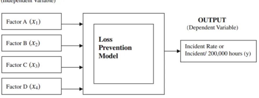
Much research is concerned with quantifying the relationship between injury prevention activities (x’s) and incident rates. Haight (2001a) established a mathematical model with multiple factors as inputs, as shown in Figure 3, and these factors are categorized as:
• Factor A --- safety awareness and motivation activities (x1).
• Factor B --- skill development and training activities (x2).
• Factor C --- new tools and equipment design methods and activities (x3).
• Factor D --- equipment related activities (x4).
Figure 3: Representation of the loss prevention system model (adapted from Haight, 2001a).
Attwood et al., (2006) established a model that can predict the frequency of the incidents and the cost associated with occupational accidents in the oil and gas industry by estimating parameters of each category such as: behavior, capability, and weather. The model was built on the concept of parallel and series reliability fault trees, as shown in figure 5. Many aspects were included in the model such as: behavior, capabilities (mental and physical), weather and safety
design. After establishing the reliability tree, they use the basic concept of reliability to calculate the time between accidents. The main difference between the work in this study and Attwood’s paper (2006) are as follow.
Attwood’s paper uses parallel and series reliability analysis to find the relationship while this study uses mainly regression analysis. Attwood’s approach (2006) uses a questionnaire to estimate model’s input confidents while in this study input factors where directly reported from actual observation. This research intends to find a proper probability density function (PDF) to utilize the forecasting techniques such as: probability outcomes, confidence intervals, prediction intervals, and the variance. Furthermore, the analyzing tools used in this research differ from previous research. In this research, the correlation between the intervention activity factors was conducted to avoid the multi-collinearity. Also, this research used moving regression to figure out if there is any influence of the time and duration of the intervention activity implementation. Previous studies did not approach the problem the same way (see Figure 4).
3.0 METHODOLOGY AND RESULTS
In this chapter, the discussion covers experimental, analytical methodologies and some of the technical details about finding a proper relationship between the injury intervention activities and incidents (y). An attempt to find a relationship between the incident and the total intervention activities is the main thrust of this research. Also, this research attempted to find the relationship between total intervention activities and incident occurrence.
3.1 REGRESSION ANALYSIS
Regression analysis is a powerful statistical tool used to estimate the parameters that are expected from a model. It is recommended to plot the dependent variable (y) versus the independent variable(s) (x’s) to get an idea of the relationship behavior (Montgomery et al., 2012). There are multiple techniques to get an appropriate model: model building techniques such as forward, backward, and stepwise regression; and transformation for dependent and/or independent variables which are used in this research in the following sections
3.1.1 Statistical indicators for evaluation
There are many indicators that can be used to assess the performance of the regression model. and mean square error ( ) are good tools to judge the performance of multiple models
(Montgomery et al., 2012).
• : Coefficient of determination which measures the variation captured by the model.
Value varies from 0 to 1. A high value is desired. It measures the variation explained by the regressors. It is calculated as shown in equation 1.
= ( 1 )
Where:
is the Sum of Square error
is the Sum of Square total
• : Mean square error, also known as residual, is a good indicator to use when
choosing among multiple models. The least value for the ( ) is preferred. is
/ (n-p) ( 2 )
Where n is the sample size
P is number of regressors + 1
• The significance of the regression test also known as the F-Test indicates the result of the hypothesis. If the result is greater than the appropriate F-table value, then the null hypothesis will be rejected based on 95 % confidence interval. Equation 3 shows the mathematical expression of the F-Test.
= ( 3 )
Where mean square error of the regression mean square error of the residual
3.2 RESULTS AND DISCUSSION
The following section contains a discussion of the results and issues faced while analyzing these data. Part one addresses the regression results and the techniques that were used to assess and enhance the relationship between the total and individual injury prevention activities (x) and incidents (y). Part two discusses the distribution fitting for the number of incidents and what is the best probability density function (pdf) using goodness of fit test.
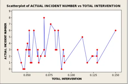
3.2.1 Incidents versus total intervention model
This section attempts to establish a relationship between incidents and total intervention activities, as opposed to attending to solely individual factors. The study begins with the working assumption that when intervention activities are implemented, incidents can be expected to decrease. The graph of incidents versus total intervention was plotted to illustrate the behavior between them. The analysis of variance for the total intervention mode shows that this assumption is invalid based on the p-value from Table 1. The total intervention activities simply are the summation of all intervention activities factor that are implemented. Using total intervention activity as one variable might be feasible in practice because the relationship is connected to the overall implemented intervention activity rather than individual factors.
Figure 5 shows an unexpected variance in the projected incident number, given the level of intervention applied. Figure 6 shows the expected behavior of the relationship between
0.150 0.125 0.100 0.075 0.050 9 8 7 6 5 4 3 2 1 0 TOTAL INTERVENTION A CT UA L IN CI D EN T NU M BE R
Scatterplot of ACTUAL INCIDENT NUMBER vs TOTAL INTERVENTION
Figure 5 : Incident number vs. total Intervention.
3.2.2 Linear regression
As discussed above, the non-linear regression was not able to fit a significant relationship between incidents and total intervention activities, so in this section a linear regression was performed to see if there is any possibility of fitting a relationship between incidents and total intervention. The model is expressed as follows:
Where:
Y number of incidents X total intervention activities
Model intercept
Coefficient of the independent variable (X)
Table 1, which presents the Analysis of Variation (ANOVA) results of the linear regression, shows that there is no relationship between incidents and total intervention. Hence, the second null hypothesis cannot be rejected. The next section follows up with a statistical analysis of the relationship between individual intervention activities and incidents. Previous
Table 1: ANOVA of total intervention.
Source DF SS MS F P
Regression 1 0.042 0.04205 0.01 0.92 Error 40 165.577 4.13942
Total 41 165.619
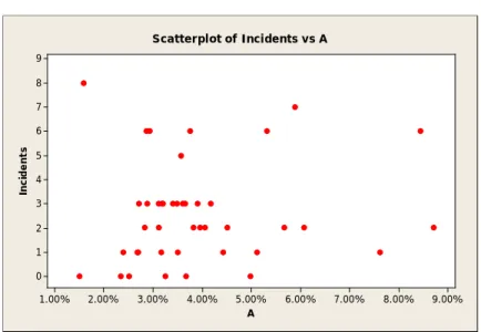
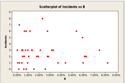
3.2.3 Scatter plot of incidents versus individual factors
One goal of a scatterplot is to find the correlation between two variables. Therefore, before performing regression analysis, incidents versus every factor were plotted as a scatterplot to see the behavior of the incidents as the intervention activity level increased. The expected behavior was to see some decline in incidents as intervention activity increased.
9.00% 8.00% 7.00% 6.00% 5.00% 4.00% 3.00% 2.00% 1.00% 9 8 7 6 5 4 3 2 1 0 A In ci de nt s Scatterplot of Incidents vs A
9.00% 8.00% 7.00% 6.00% 5.00% 4.00% 3.00% 2.00% 1.00% 0.00% 9 8 7 6 5 4 3 2 1 0 B In ci de nt s Scatterplot of Incidents vs B
Figure 8: Incidents versus Factor B.
0.50% 0.40% 0.30% 0.20% 0.10% 0.00% 9 8 7 6 5 4 3 2 1 0 C In ci de nt s Scatterplot of Incidents vs C
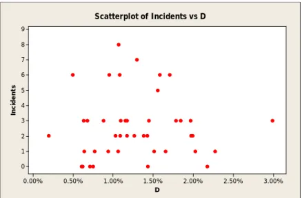
3.00% 2.50% 2.00% 1.50% 1.00% 0.50% 0.00% 9 8 7 6 5 4 3 2 1 0 D In ci de nt s Scatterplot of Incidents vs D
Figure 10: Incidents versus Factor D.
It appears from Figure 7 through Figure 10 that there is no such relationship as that anticipated in section 3.2.1. In addition, there is randomness to the pattern because while it was expected there would be fewer incidents as the intervention increased, there was actually an increase in incidents as the intervention increased. This pattern might be due to collinearity between intervention factors. One way to investigate the correlation between the independent variable is to plot intervention factor versus each one and calculate the correlation factor which is discussed in section 3.2.4.
3.2.4 Correlation between regressors
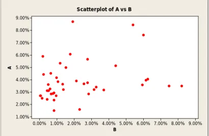
As discussed in section 3.2.3, the multi-collinearity among the intervention factors might have distracted from the relationship between the incidents and intervention activities. In order to verify that there is such a relationship, a scatterplot was used to visualize the pattern between the regressors. 9.00% 8.00% 7.00% 6.00% 5.00% 4.00% 3.00% 2.00% 1.00% 0.00% 9.00% 8.00% 7.00% 6.00% 5.00% 4.00% 3.00% 2.00% 1.00% B A Scatterplot of A vs B
Figure 11: Factor A versus factor B.
9.00% 8.00% 7.00% 6.00% 5.00% 4.00% 3.00% 2.00% A Scatterplot of A vs C
0.50% 0.40% 0.30% 0.20% 0.10% 0.00% 9.00% 8.00% 7.00% 6.00% 5.00% 4.00% 3.00% 2.00% 1.00% 0.00% C B Scatterplot of B vs C
Figure 13: Factor B versus factor C.
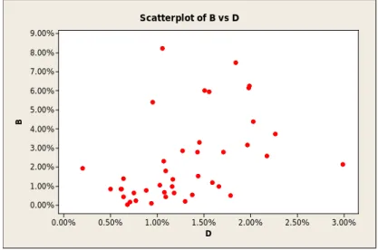
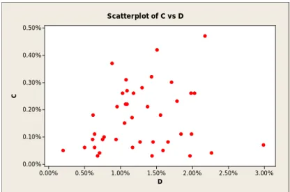
Figure 11 reveals a pattern that indicates that factor A and B might be correlated to each other. This correlation might have inversely affected the estimation of the parameters in the regression model or the significance of the model due to the inflation of the variance (Montgomery et al., 2012). 3.00% 2.50% 2.00% 1.50% 1.00% 0.50% 0.00% 9.00% 8.00% 7.00% 6.00% 5.00% 4.00% 3.00% 2.00% 1.00% 0.00% D B Scatterplot of B vs D
3.00% 2.50% 2.00% 1.50% 1.00% 0.50% 0.00% 0.50% 0.40% 0.30% 0.20% 0.10% 0.00% D C Scatterplot of C vs D
Figure 15: Factor C versus factor D.
All of Figure 11 through Figure 15 show that some input variables correlate with each other; however, to assure that there are indeed such correlations, regression analysis was conducted to see if some significant value could be found that could easily judge the collinearity.
Table 2: P-value for the inputs versus each other.
Input/response B C D
A 0.077 0.165 0.836
B - .395 .004
C - - .285
Table 2 shows that there is a relationship between factor B with both A and D (based on 90% C.I.). In cases of multi-collinearity, it is recommended to remove the correlated factor and see
Where Y = number of incidents
Table 3: Minitab result for the model including all the factors.
Predictor Coef. SE Coef. T P Constant 1.845 1.198 1.54 0.132 A 11.11 22.62 0.49 0.626 B -1.93 17.80 -0.11 0.914 C 204.4 304.9 0.67 0.507 D 1.44 66.96 0.02 0.983 S = 2.16855 R-Sq = 2.3% R-Sq(adj) = 0.0% Analysis of Variance Source DF SS MS F P Regression 4 4.123 1.031 0.22 0.926 Residual Error 37 173.996 4.703 Total 41 178.119
Table 3 shows that the model and all the regressors are insignificant and the value of R^2 is extremely low. Based on this model, the null hypothesis 1 can be accepted and the conclusion is there is no relationship between incidents and intervention activity. In the previous research the multi-collinearity was not addressed which might affect the significance of the model. Also, the previous research used higher polynomial factors and interaction between regressors which provided a more significant model, but it can be considered as over fitting and the model may have lost some degrees of freedom due to the addition of too many input factors.
As discussed in section 3.2.4, the correlation between regressors might affect the model and make it insignificant. To solve this problem, Factor B was removed from the model and the new regression model included Factors A, C and D only. After getting a significant model, the optimization of the resources can be conducted. The idea of removing the correlated factor is that one regressor can be explained and represented by another regressor. The proposed model is:
Where Y = number of incidents
Table 4: MATLAB results for the model including all the factors excluding factor B.
Table 4 shows that the model without factor B is still shows an insignificant relationship (P-value 0.814). So the same conclusion can be drawn as for the previous model: a relationship between incidents and intervention activity cannot be achieved. Further analysis is needed to investigate the relationship.
Again, as intervention activities are implemented to reduce the number of incidents, rather than observing a decline in the incidents, we observe an increase. This further strengthens
Source DF SS MS F P
Regression 3 4.322 1.441 0.32 0.814
Residual 38 173.797 4.574
Table 5: All possible combinations of regression model. Factors P-Value A 0.512 B 0.902 C 0.391 D 0.914 AB 0.807 AC 0.602 AD 0.806 BC 0.696 BD 0.991 CD 0.695 ABC 0.881 ABD 0.869 BCD 0.932 ABCD 0.926
As shown in Table 5, no significant model was found for the all possible subsets of factors. In order to determine if there is indeed any relationship, a moving regression will be conducted to see if there is any influence of the time of the collection of data. At this stage, multiple lengths of moving regressions were performed to check for any chance of capturing a relationship that might have been affected by the time of collecting data or the duration. To do so, the ‘linest’ function was used which is a built-in function in excel© to find both the value of
36 32 28 24 20 16 12 8 4 1.0 0.8 0.6 0.4 0.2 0.0 Model V al ue R-square P-value Variable Time Series Plot of R-square and P-value
Figure 16: Value of and using 6 points.
As shown in Figure 16, there is no sign of a significant model except for with the two points that happened almost at the end. The patterns of both and the are random,
33 30 27 24 21 18 15 12 9 6 3 0.9 0.8 0.7 0.6 0.5 0.4 0.3 0.2 0.1 0.0 Model V al ue R-square P-Value Variable Time Series Plot of R-square, P-Value
Figure 17: Value of and using 9 points.
30 27 24 21 18 15 12 9 6 3 1.0 0.8 0.6 0.4 0.2 0.0 Model V al ue R-square P-value Variable Time Series Plot of R-square, P-value
As shown in the above figures, there is no significant model and also the patern R^2 and P-value are random and no relationship can be detected when the significance level is not met However, in the middle of the moving regression, for all used points, there is a pattern of improvement in both R^2 and P-value . This means there is a possibility to have a significant model in the case of using half of the data. Figure 19 shows that the case of using half the point of the sample size and unfortunately there is no relationship and actually the previous attempts are better. In the end, the conclusion is that there is no relationship between incidents and intervention activities.
18 16 14 12 10 8 6 4 2 1.0 0.8 0.6 0.4 0.2 0.0 Model V al ue R-square P-value Variable Time Series Plot of R-square, P-value
3.2.5 Natural logarthim transformation model
In many cases, linear regression cannot be fitted easily due to the complexity of the relationship between inputs and response. One solution for this problem is to find a proper transformation for response, inputs or both of them. Based on the pattern and behavior seen in previous section, it is good to check logarithm transformation linearization. Equation 4 shows the expected relationship of the exponential function.
( 4 )
Where:
Y: number of incidents
X: implemented intervention activities
Equation above can be linearized by making a logarithm transformation, then the relationship will be as in Equation 5.
( 5 ) Where:
Y: number of incidents
X: implemented intervention activities Model intercept
-2.50 -2.75 -3.00 -3.25 -3.50 -3.75 -4.00 -4.25 2.5 2.0 1.5 1.0 0.5 0.0 ln(A) ln (i nc id en ts )
Scatterplot of ln(incidents) vs ln(A)
Figure 20: scatterplot of ln( Incidents) vs ln (A).
-2 -3 -4 -5 -6 -7 -8 2.5 2.0 1.5 1.0 0.5 0.0 ln(B) ln (i nc id en ts ) Scatterplot of ln(incidents) vs ln(B)
-5.0 -5.5 -6.0 -6.5 -7.0 -7.5 -8.0 -8.5 2.5 2.0 1.5 1.0 0.5 0.0 ln( C) ln (i nc id en ts ) Scatterplot of ln(incidents) vs ln( C)
Figure 22: scatterplot of ln( Incidents) vs ln (C).
-3.5 -4.0 -4.5 -5.0 -5.5 -6.0 -6.5 2.5 2.0 1.5 1.0 0.5 0.0 ln(D) ln (i nc id en ts ) Scatterplot of ln(incidents) vs ln(D)
Figure 20 through Figure 23 show that there is no pattern of linear relationship between the incidents and intervention activities even after making the transformation. To avoid the problem of taking the logarithm of zero, box-cox transformation suggests that adding two parameter transformations to solve the logarithm of zero as shown on Equation 6.
( 6 )
Table 6: Regression result with natural logarithm for the response.
The regression equation is
Ln(y+1) = - 1.86 + 0.221 ln(a) + 0.0019 ln(b) + 0.110 ln(c) + 0.086 ln(d)
Predictor Coef SE Coef T P Constant -1.859 2.567 -0.72 0.473 lna 0.2207 0.2800 0.79 0.436 lnb 0.00192 0.09343 0.02 0.984 lnc 0.1101 0.1306 0.84 0.405 lnd 0.0862 0.2200 0.39 0.697 S = 0.633073 R-Sq = 5.6% R-Sq(adj) = 0.0% Analysis of Variance Source DF SS MS F P Regression 4 0.8747 0.2187 0.55 0.703 Residual Error 37 14.8289 0.4008 Total 41 15.7036
Table 6 showed the results of the regression model after taking the natural logarithm for both the response and the predicted variables. Unfortunately, the model is insignificant, with a p-value of 0.703. Which means it couldn’t be determined that variations in the occurrence of incidents cannot be explained by variations in the intervention activities.
3.3 DISTIRBUTION FITTING FOR INCIDENTS
As shown in Figure 24, there is a semi-positively skewed pattern on the number of incidents. While the incidents can be counted as discrete (number of incidents), many distributions can be fitted to these data as a probability density function (pdf).
8 6 4 2 0 12 10 8 6 4 2 0 incidents Fr eq ue nc y Histogram of incidents
To begin with, Poisson distribution have chosen to apply. The Poisson distribution is appropriate for applications that involve counting the number of times random event occurs in a given amount of time, distance, area, etc. Here, incidents are assumed to be a random variable. Knowing the probability distribution of this random variable provides important statistical estimates for the incidents such as the expected number of incidents, the variance, and the mode.
Equation 7 shows the probability density function of the Poisson distribution. The maximum likelihood estimator for Poisson distribution is the average, as shown in Equation 7. Therefore, to find the events outcome probability for incidents, the parameter (mean) should be estimated. The proof for this hypothesis was conducted and the results are shown in section 3.3.2.
( 7 )
Where
i= week
x = number of incidents in week i
n= sample size
3.3.1 Goodness of fit test
This test was performed with 9 classes (sample size n = 42) to make every event a random event. The critical value of chi-square was 15.507 (using 95% C.I.), however only with the first two classes combined and the last five classes combined to end with 4 classes and chi-square from the table is 5.99. Table 7 shows the values of the observed and expected data. The expected value of the outcome was computed using Equation 8. The test value was calculated using Equation 9.
Ei pi ( 8 )
( 9 )
Where
E = number of expected for every outcome O = number of observed for every outcome
Table 7: Chi-square test for Dist. Fitting.
Observed Expected O combined E combined (E-o)^2/E
0 6 3.13438 14 11.26884 0.532801 1 8 8.134463 2 9 10.55543 9 10.55543 0.26882 3 11 9.131289 11 9.131289 0.317462 4 0 5.924467 8 10.76765 0.957487 5 1 3.075081 6 5 1.115 7 1 0.49313 8 1 0.159974 Total 2.07657 3.3.2 Test of hypothesis
H0: The incident follows Poisson distribution
H1: The incident does not follow Poisson distribution
The critical value is 5.99, thus null cannot be rejected (it’s accepted), and the incidents follow Poisson distribution based on the dataset used. The importance of the Poisson distribution is highly related to the passion process which is a universal stochastic process that can be very helpful in estimating the long term behavior of incidents occurrence.
4.0 CONCLUSIONS AND FURTHER WORK
4.1 ANALYTICAL SUMMARY
To summarize, with this research, the researcher intended to find a relationship between intervention activities and incidents. A linear model using all factors as regressors yielded an insignificant result, with a p-value of 0.9.
The method of combining all possible regressors was conducted, but all of the computed models yielded insignificant results. Linear models based on a moving range of data points was conducted to check if a subset of the data could provide a better and significant model. After trying different ranges, all of the generated models were still insignificant.
A linear model was also built using natural logarithm transformation on the data, but it, too, was insignificant. Therefore, after analyzing the data using several different regression modelling techniques, it can be concluded that a relationship between incidents and intervention activities does not exist based on the data set and the modeling techniques used. This work further illustrates the complex nature of preventing work place injuries. More research is needed in this area to help safety practitioners manage more thoroughly and with more clearly, the complicated process of implementing a health and safety management system.
4.2 LIMITATIONS
Data collection is a critical step for a model; unfortunately, the researcher was involved in neither the design of the original model nor the data collection. That prevents the researcher from knowing the foundation conditions and environment where the incidents and the work towards their prevention occurred.
The results for this study are based on the dataset used, meaning the results cannot be generalized to the safety field. Using the fitted Poisson distribution is valid for this particular data set and might not be valid for others. Also, the amount of data analyzed was limited, so if there were more, the results might be different.
4.3 SUGGESTIONS FOR FUTURE WORK
It would be a positive step to include some indicator variables that can be classified based on the individual (i.e. level of training, weight, and age). These variables might give a better understanding of the loss prevention programs and how to allocate the resources properly (Burke et al., 2011). In reality, cost is a critical limitation, so including cost in the model would be beneficial for decision makers when making decisions about allocating funds towards injury prevention activities.
REFERENCES
ABDEL-ATY, M. A. & RADWAN, A. E. 2000. Modeling traffic accident occurrence and involvement.
Accident Analysis & Prevention, 32, 633-642.
BURKE, R. J., CLARKE, S. & COOPER, C. L. 2011. Occupational Health and Safety, Abingdon, Oxon, GBR, Gower Publishing Limited.
CHOPRA, S. & MEINDL, P. 2007. Supply chain management. Strategy, planning & operation, Springer. HAADIR, S. A. & PANUWATWANICH, K. 2011. Critical Success Factors for Safety Program
Implementation among Construction Companies in Saudi Arabia. Procedia Engineering, 14, 148-155.
HAIGHT, J. M., R. E. THOMAS, L. A. SMITH, R. L. BULFIN JR. AND B. K. HOPKINS 2001.
Intervention Effectiveness Research: Phase 1, Developing a Mathematical Relationship between Interventions and Incident Rates for the Design of a Loss Prevention System.
American Society of Safety Engineers Technical Forum, 38-44.
HAIGHT, J. M., THOMAS, R. E., L. A. SMITH, BULFIN, R. L. & HOPKINS., B. K. 2001b. Intervention Effectiveness Research:Phase 2 Design, Optimization & Verification of the Loss Prevention System & Analysis Models. Professional Safety - The Journal of the America Society of Safety Engineers, 33-37.
IYER, P. S., HAIGHT, J. M., DEL CASTILLO, E., TINK, B. W. & HAWKINS, P. W. 2005. A research model—forecasting incident rates from optimized safety program intervention strategies. Journal of Safety Research, 36, 341-351.
Iyer, Parameshwaran S., et al. "Intervention effectiveness research: Understanding and optimizing industrial safety programs using leading indicators." Chemical Health and
Safety 11.2 (2004): 9-19.
LEIGH, J. P., WAEHRER, G., MILLER, T. R. & KEENAN, C. 2004. Costs of occupational injury and illness across industries. Scandinavian journal of work, environment & health, 199-205.
MONTGOMERY, D. C., PECK, E. A. & VINING, G. G. 2012. Introduction to linear regression
OYEWOLE, S. A., HAIGHT, J. M., FREIVALDS, A., CANNON, D. J. & ROTHROCK, L. 2010. Statistical evaluation and analysis of safety intervention in the determination of an effective resource allocation strategy. Journal of Loss Prevention in the Process Industries, 23, 585-593. SHAKIOYE, S. O. & HAIGHT, J. M. 2010. Modeling using dynamic variables – An approach for the
design of loss prevention programs. Safety Science, 48, 46-53.
WACHTER, J. K. & YORIO, P. L. 2014. A system of safety management practices and worker engagement for reducing and preventing accidents: An empirical and theoretical investigation.