The Semi-blind Source Extraction Algorithm for
Array Radar Signal
Gang Wang, Nini Rao∗, Xiaochuan Du, Feng Ou, Caiquan Liu, and Guogong Xu University of Electronic Science and Technology of China, Chengdu 610054, China
*Corresponding author email: [email protected]
Chaoyang Qiu
Institute of Leihua Electronic Technology, Wuxi, 214063, China
Abstract⎯A semi-blind source extraction algorithm for noisy mixtures based on a linear predictor is proposed. The novel algorithm is firstly validated using the benchmark data and then is applied to extract array radar signal suffering from jamming interference. The results showed that the novel algorithm can effectively extract the target signal in radar echo. Thus, it has practical application prospect in array radar for increasing anti - jamming interference ability.
Index Terms⎯blind source extraction, cost function, AR autoregressive model parameter, array radar, jamming interference
I. INTRODUCTION
Blind source extraction (BSE) is a kind of blind source separation (BSS) technology [1] and has become a research hotspot in fields of signal processing in recent years. The purpose of BSE is to estimate a small subset of source signals, which are linear combination of all observed signals. Compared with BSS, BSE has more advantages, and has wider applications in many fields such as radar array signals processing [2], biomedical signal processing [3-4]and speech processing [5].
So far, a lot of BSE algorithms have been proposed. The typical algorithms included those based on the high order statistics (HOS) [6-7] and the second order statistics(SOS)[8]. Since the algorithms exploiting HOS have high computational load, the SOS-based algorithms is developed using priori knowledge about signal’s temporal structure. However, the SOS algorithms based on linear predictors [9-12] required that all source signals are not correlated with each other and each source signal has different temporal structure.
Liu et al. [10] first proposed to extract the desired signal from mixtures when the AR model parameters of this signal were known in the noise-free case and then extended the results to the noisy case [13]. The algorithms of Liu et al. [10, 13] are classified as the mean cross prediction error (MCPE) algorithms that can extract the signal with minimal MSPE. In our previous work [14],
we proposed a BSE algorithm whose cost function can cater for the specific AR model parameters of desired signal. Our algorithm [14] is classified as the mean square cross prediction error (MSCPE) algorithm that can extract the signal with minimal MSCPE in the noise-free case. Our previous research results showed that the desired signal has always minimal MSCPE, but has not minimal MSPE.
Following Liu’s research ideas [10, 13], we extend the algorithm in noise - free case in [14] to a novel BSE algorithm in the noisy case and apply the novel algorithm to extract array radar signal in this paper.
This paper is outlined as follows: In section II, the novel algorithm with new cost function in noisy case is introduced. The application feasibility of novel algorithm in array radar is analyzed in section III. The numerical results using the benchmark data and synthetic array radar signals are given and analyzed in section IV. The conclusions are finally drawn in section V.
II. ALGORITHM
In the noise-free case [14], we supposed that an observed stochastic signal vector x with m-dimension is the linear mixture of an l-dimensional zero-mean and unit-variance vector s, that is,
x(n)=As(n)
where A ∈Rmxl is an unknown mixing matrix. To suit for the ill conditioned case (m>l) and to make the novel algorithm be simpler and faster, the observed signals x need to be pre-whitened, i.e., HE{xxT}HT=I, where H∈Rlxm is a pre-whitening matrix. However, we assume that x has been pre-whitened and A is an orthonomal matrix in this section for convenience.
On the basis of hypotheses above, we have the following signal models in the noisy case:
x(n) = As(n) +v(n) = x(n) +v(n)
(1) where x(n)∈R m is the observed stochastic signal vector with m-dimension in the noisy case and v(n) is an unknown additive Gaussian white noise. Here we still assume that l is less than m.
The observation correlation matrix is calculated as follows:
C=E
{
x(n)xT(n)}
=ACsAT +σ2I (2)Manuscript received July 27, 2011; revised November 12, 2011; accepted December 9, 2011.
Let λi and ui (i=1,2,...,m) be respectively the eigenvalue and the orthonormal eigenvector of C corresponding to λi. The C can be decomposed as:
C=UΣUT
whereΣ=diag(λ1,λ2,",λm)and U=
(
u1,u2,"um)
. Since l is less than m, the no increasingly ordered eigenvalues can be expressed as:2 1
1 λ λ λ σ
λ ≥"≥ l > l+ ="= m = (3)
Thus, the subspaces of signal and noise are respectively
[
l]
s
u
u
U
=
1,
⋅
⋅⋅
,
andU
v=
[
u
l+1,
⋅
⋅⋅
,
u
m]
(4)The variance σ2 of v(n) can be estimated by the noise subspace and the observation data x can be projected into
the signal subspace through UTs x.
For convenience, we also assume that A and v(n) in (1) have been projected into the signal subspace in the noisy case.
In the presence of noise, the noise influences must be removed so that the resulting cost function remains same form with that in noise-free case [14].
The goal of BSE is to find a vector w that makes y(n)=wTx(n)=wTAs(n)+ wTv(n) be an estimated source signal with additive noise. For the noise v(n), we have
[
]
{
}
{
}
{
}
1 2 l
2
( ) v ( ), v ( ), , v ( ) ( ) ( ) σ , ( 1,2, , )
( ) ( ) 0, ( 1,2, , )
( ) ( ) 0, ( 1,2, , )
i i
i j
i j
n n n n
E v n v n i l
E v n v n i j, i, j l
E s n v n i, j l
= ⋅⋅⋅ = = ⋅⋅⋅ = ≠ = ⋅⋅⋅ = = ⋅⋅⋅ T v (5)
where σ2 is the variance of noise. Assume that
v(n) w u(n) u(n) y(n) v(n) w y(n) (n) x w (n) y x(n) w y(n) T T T T = + = + = = = (6)
Thus, the instantaneous noisy prediction error (PE) (denoted by e(n)) can be calculated as:
T
T
( ) ( ) ( )
( ) ( 1), ( 2), , ( )
e n y n n
n y n y n y n p
= −
⎡ ⎤
=⎣ − − ⋅⋅⋅ − ⎦
b Y
Y (7)
where b is the AR parameters of a desired signal. Then, we utilize e(n) to estimate e(n) (the PE in noise - free case in [14]) since e(n) is unknown.
Let eu(n) denote the instantaneous PE of noise u(n), that is,
T u
T
( ) ( ) ( )
( ) [ ( 1), ( 2), , ( )]
e n n n
n n n n p
= −
= − − ⋅⋅⋅ −
u b u
u u u u (8)
Then, we have:
) ( ) ( )
(n en e n
e = + u (9) The new cost function in noisy case is designed as:
(
)
{
}
(
)(
)
{
e(n) e (n) e(n q) e (n q)}
, 0 q p E min q) e(n)e(n E min ) J( u u 2 w 2 w ≤ < − − − − = − = w (10) where q denotes error delay.A novel BSE algorithm in noisy case can be constructed using eigenvalue decomposition (EVD) and the new cost function in (10). Assume that
⎟ ⎟ ⎠ ⎞ ⎜ ⎜ ⎝ ⎛ − − = ⎟ ⎟ ⎠ ⎞ ⎜ ⎜ ⎝ ⎛ − − =
∑
∑
= = p 1 i i v p 1 i i i) (n b (n) (n) i) (n b (n) (n) z v v z x x (11)By combining (6) and (11), we have:
w z z w e w z z w e z z z T v v T v T T v ) ( ) ( ) ( ) ( ) ( ) ( ) ( ) ( ) ( n n n n n n n n n = = = = + = (12) Assume that
{
(n) (n q)}
E(q)= z zT −
Z (13) Thus, Z(q) can be expressed as follows:
{
}
(
)(
)
{
}
{
} {
}
(
)
{
(n) (n q)} (
E{
(n) (n q))
}
E q) (n (n) E q) (n (n) E q) (n q) (n (n) (n) E q) (n (n) E (q) T v v T v T v T T v v T − + − − − − − = − − − − = − = z z z z z z z z z z z z z z Z (14)
Note that z(n) is determined by the source signal and zv(n) is determined by noise. Further, we have:
{
}
{
n n q} {
E n n q}
-b bb IE q n n E 2 i ⎟⎟σ
⎠ ⎞ ⎜ ⎜ ⎝ ⎛ + = − = − = −
∑
− = + q p i q i q T v v T v T v z z z z z z 1 ) ( ) ( ) ( ) ( 0 ) ( ) ( (15) Z(q) can be simplified as:{
} (
{
)
}
{
(n) (n q)}
-b bb σ IE q) (n (n) E q) (n (n) E (q) 2 q p 1 i q i i q T T v v T ⎟ ⎟ ⎠ ⎞ ⎜ ⎜ ⎝ ⎛ + − − = − − − =
∑
− = + z z z z z z Z (16)From (16), we can know that Z(q) is calculated using the observed data x(n) and AR model parameters b of desired signal. Thus, the algorithm with new cost function in noisy case can finally be expressed as:
{
}
{
( ) ( )}
{
( )}
) ( ) ( ) ( ) ( ) ( ) ( 1 q MINSVD q q MINEVD b b b -q n n q i n n n 2 q p 1 i q i i q Z Z Z w z z E Z x b x z T T p i i = = ⎟ ⎟ ⎠ ⎞ ⎜ ⎜ ⎝ ⎛ + − − = ⎟ ⎟ ⎠ ⎞ ⎜ ⎜ ⎝ ⎛ − − =∑
∑
− = + =σ (17)
where the normalized eigenvector corresponding to the minimal eigenvalue of Z(q)ZT(q) is calculated by the MINEVD { Z(q)ZT(q)} and the normalized singular vector corresponding to the minimal singular value of Z(q) by the MINSVD{ Z(q)}.
III. APPLICATIONS IN ARRAY RADAR SUFFERING FROM JAMMING INTERFERENCE
instantaneously mixed noisy signal. The difference between the desired target signals in radar echo and its transmitted signals mostly lies on time delay and frequency slide, and thus the AR model parameters of the desired target signals can be estimated using the transmitted signals. According to the above analysis, our novel algorithm in noisy case can be applied to extract the desired target signals received by array radar [15-18] for increasing the detection ability of array radar under the jamming interference environment.
For an array radar system suffering from jamming interference, the signal model mainly consists of target signals, jamming interference signal and noise [16]. In practice, the forms of transmitted radar signals are very abundant. Here assume that the transmitted radar signal, denoted by st, is a standard amplitude modulation (AM) signal, that is,
st(n)=B0
[
1+kAMrm(n)]
cos(
2πf0n)
(18)whereB0andkAMare respectively the amplitude and the modulation coefficient of transmitting signal, f0 is the carrier frequency, and rm(n) is the modulation signal. Assume that the time delay is Δτ and the frequency slide is Δf . So the received target signal denoted by se can be expressed as follows:
(
)
(
)
'
1 AM 0
( ) 1 ( ) cos 2π
e m
s n =B ⎡⎣ +k r n ⎤⎦ f + Δf n+ Δτ (19) where B1 and
k
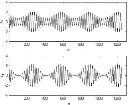
AM' are respectively the amplitude and the modulation coefficient of target signal received.The received target signal se and transmitted radar
signal st produced by (18) and (19) are shown in Fig. 1.
Figure 1. The received (upper) and transmitted (down) radar signals
There are also plenty of kinds of jamming interference signal forms. The noise modulation jamming interference signals [16-17] are considered in this paper. The noise modulation are further divided into noise amplitude modulation (AM), noise frequency modulation (FM) and noise AM-FM, etc. Noise FM jamming interference signals denoted by sf. were adopted here and its signal
model is denoted as:
( )
( )
⎥⎦ ⎤ ⎢
⎣ ⎡
Δ +
=
∑
'
' ' 0cos 2
n n FM j
f n U f n k u n n
s
π
(20)where
u
n( )
n
' is the modulation noise. We assume that it is Gaussian white noise with the limited band and the variance σf2.k
FM is the frequency modulation coefficient.Assuming that array radar has m receiving antenna (or channels), the received radar signal can be modeled as follow:
x’(n) = A’s’(n) + v’(n) (21)
where x’(n) is the observed signals of radar; s’(n) is the
source signals including the received target signal, jamming interference signal and noise, etc; v’(n) is an
unknown additive Gaussian white noise. Since A’ is the
results that antenna responds to narrow band signal on certain direction in array radar, it is a mixture matrix.
It is easy to find that the received radar signal model in (21) is same with the BSE model in (1). Thus the extraction of the radar target signal from the signals received by array radar is a BSE problem.
IV. NUMERICAL RESULTS
A. The Benchmark Data
In this subsection, two experiments are performed to demonstrate the validity of novel algorithm. We use the benchmark data with three source signals: s1, s2 and s3, as
shown in Fig.2. They can be found in the file ABio7.mat provided by ICALAB toolbox in [1]. In our experiment, we define the signal - to - noise ratio (SNR) as follows:
(
2 2)
10log 10 σs σ
=
SNR (22) where 2
s
σ and σ2 respectively denote the variance of
signal and noise. In the first experiment, we fixed the SNR at 15dB, and compared our novel algorithm with the algorithm in [13]. In the second experiment, we extracted the desired signal under different SNR.
Figure 2. Three source signals in Benchmark data (l=3)
and calculated the AR model parameters of si (i=1, 2, 3) using Matlab function ‘aryule’. As we have one more mixture than the number of sources, this additional degree of freedom was used to estimate the variance, σ2, of the additive Gaussian white noise that is determined by SNR. For easily calculating the SNR and keeping good algorithm performance, we normalized A into an orthonomal matrix. The performance index (PI) of desired signal si (i=1, 2, 3) are defined to evaluate the performance of novel algorithm, that is,
⎟⎟ ⎟ ⎠ ⎞ ⎜⎜
⎜ ⎝ ⎛
⎟ ⎟ ⎠ ⎞ ⎜
⎜ ⎝ ⎛
− −
=
∑
=
1 1
1 log 10 ) (
1 2 2 10
l
j i
j
g g l
i
PI (23)
where g = wTA= [g1, g2, g3]T is the global vector and is
normalized as gT g=1. Generally speaking, an algorithm is evaluated to have good performing if the PI of extracted signal is below -30 dB[10].
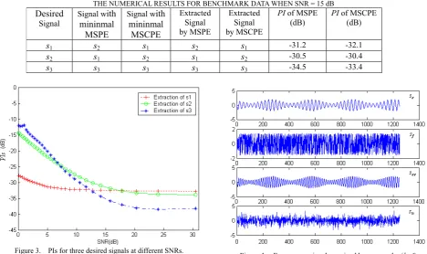
The numerical results when SNR =15dB in the first experiment were summarized in Table 1. The results confirmed that the MSPE algorithm extracted the signal with minimal MSPE and our algorithm extracted the signal with minimal MSCPE. Two algorithms can extract the signal based on the viewpoint for extracting a signal because all PIs for two algorithms in table 1 are below -30dB. However, the extracted signal with minimal MSCPE exactly corresponds to the desired one in the experiments, while the MSPE algorithm just did that in the third dataset. The results demonstrated that our algorithm performed better. The experiment results further verified that the desired signal has minimal MSCPE, but has not minimal MSPE.
In the second experiment, assume that s1, s2 and s3 are
respectively the desired signals, and the novel algorithm and AR model parameters corresponding to the desired signal are used to extract the desired signal at different SNRs. For each fixed SNR, we performed 100 different runs and averaged the value of the PIs.
The numerical results are summarized in Fig 3. We found that PIs for three desired signals are less than -30 dB when SNR is more than 15 dB from Fig. 3. When s1
was used as the desired signal, the novel algorithm can extract this signal successfully even at SNRs = 5 dB. Two experimental results validated our algorithm.
B. The Array Radar Data
In this simulation, we assumed that the sources in (21) consisted of four kinds of signals: the received target signal se with AM, FM noise jamming interference signal sf, Gaussian white noise sn and the reference target signal see whose carrier frequency is different from se. see is set to evaluate the extraction ability of novel algorithm. Assume p=10, m=5, l=4. One more mixture than the number of sources was used
to estimate the variance of the additive Gaussian white noise v’(n). It is reasonable to assume that there are more
receiving sensors than sources in practice. The above four source signals and their mixture with v’(n) are shown in
Fig. 4 and Fig. 5 respectively.
TABLE I.
THE NUMERICAL RESULTS FOR BENCHMARK DATA WHEN SNR = 15 dB Desired
Signal Signal wmininmal ith
MSPE
Signal with mininmal
MSCPE
Extracted Signal by MSPE
Extracted Signal by MSCPE
PI of MSPE (dB)
PI of MSCPE (dB)
s1 s2 s1 s2 s1 -31.2 -32.1
s2 s1 s2 s1 s2 -30.5 -30.4
s3 s3 s3 s3 s3 -34.5 -33.4
Figure 3. PIs for three desired signals at different SNRs.
Figure 5. Mixtures of source signals with additive Gaussian white noise (m=5)
In this study, we extracted the received target signal se
from the mixtures by means of AR model parametersof st because se is the echo of st and it is difficult to calculate the AR model parametersof se in practice. The performance of novel algorithm is estimated using the correlation coefficient (CC) between the extracted target signal denoted by s’e and se, that is,
CC
=
s
e,
s
'es
e,
s
es
e',
s
'e (24)where operator <.> denotes the inner product, and CC is the correlation coefficient between “0” and “1”.
We executed Monte Carlo simulations under the different time delays, frequency slides and SJNRs (Signal - to - Jamming and Noise ratio, SJNR) ranging from zero to 30 dB. The results showed that the average CC exceeds 0.8 when taking SJNR > 15 dB and q = 2. This result illustrated that our algorithm can successfully extract the target signal under the jamming interference and noise environment. Further, we adopted the BSS method based on fast-ICA algorithm [16-17]to process the mixtures in Fig. 5. The similar results with our algorithm are obtained (Fig.6). However, our algorithm only extracted one desired signal, while BSS method separated all source signals. Thus, our algorithm has better real-time property compared with BSS method.
V. CONCLUSIONS
In this paper, a novel semi-BSE cost function based MSCPE is proposed on the viewpoint of extracting a desired signal from instantaneous noisy mixtures. Theoretical analysis and computer simulations using the benchmark data showed that the novel algorithm can extract any desired signal using its AR model parameters and embody the desired property.
The novel algorithm in noisy case was applied in the extraction of target signal received by array radar suffering from jamming interference. The numerical results confirmed that it can well extract the target signal from the received radar signals under the condition of SJNR > 15dB and q = 2 and has better real-time property
compared with BSS method.
Thus, this work showed that the algorithm based on MSPCE indeed works better than that based on MSPE in noisy case. The proposed algorithm has practical application prospect in array radar for increasing anti - jamming interference ability.
Figure 6. The performance comparisons between our algorithm and the BSS method
ACKNOWLEDGMENT
This work was supported in part by a grant from Aeronautical Science Foundation of China (Grant No.
20112080014).
REFERENCES
[1] A. Cichocki, S. Amari, et al. Adaptive Blind Signal and Image Processing. Jonh Wiley &Sons, Inc., New York, 2003.
[2] A. Hyvarinen, J. Karhunen, E. Oja. Independent Component Analysis. Jonh Wiley &Sons, Inc., New York, 2003. [3] Y. L.Ye, C –Y. Sheu Phillip, et al, “An efficient semi-blind
source extraction algorithm and its applications to biomedical signal extraction,” Science in China, Series F: Information Sciences, Vol.52, No.2, pp.1863-1874, 2009. [4] C. L.Li and G. S. Liao, “A reference-based blind source extraction algorithm,” Neural computing & applications, Vol.19, No.2, pp.299-303, 2010.
[5]W. Gang, C. G. Li, L.Dong, “Noise estimation using mean square cross prediction error for speech enhancement,”
IEEE Transactions on Circuits and Systems-I, Vol.57, No.7, pp.1489-1499, 2010.
[6] M.G.Jafari, et al., “Sequential Blind source separation based exclusively on second order statistics developed for a class of periodic signals,” IEEE Trans. Signal Process,Vol.54, No.3, pp. 1028-1040, 2006.
[7] A. Cichocki, T.Rutkowski, A.K.Barros and S. H.Oh, “Blind Extraction of Temporally Correlated but Statistically Dependent Acoustic Signals,” Proc. IEEE Workshop on Neural Networks for Signal Processing,, Sydney, Australia, pp.455-464, 2000.
[8] R. R.Gharieb, A.Cichocki, “Second-order statistics based blind source separation using a bank of subband filters,”
Digital Signal Processing, Vol.13, No.2, pp.252-274, 2003.
temporally correlated sources using second order statistics,” Neural Processing Letters, Vol.12, pp.91-98, 2000.
[10] W.Liu, D.P. Mandic, A.Cichocki, “A class of blind source extraction algorithms based on a linear prediction,” IET Signal Processing, Vol.1, No.1, pp.29-34, 2007.
[11] A.K.Barros, A.Cichocki, “Extraction of specific signals with temporal structure, Neural Computation,” Vol.13, No.9, pp.1995-2000, 2001.
[12] Z.L.Zhang, Y. Zhang, “Robust extraction of specific signals with temporal structure,” Neurocomputing, Vol.69, pp.888-893, 2006.
[13] W.Liu, D.P.Mandic, A.Cichocki, “Blind Second-Order Source Extraction of Instantaneous Noisy Mixtures,”
IEEE Trans. CAS II: Express Briefs, Vol.53, No.9, pp.931-935, 2006.
[14] G.Wang, N.Rao, S. J. Shepherd and C. B. Beggs, “Extraction of Desired Signal Based on AR Model with its Application to Atrial Activity Estimation in Atrial Fibrillation,” EURASIP Journal on Advances in Signal Processing, Article ID 728409, 2008.
[15] W. Xiao, X. Zhang, S. Du, “Blind Separation of Radar Signals,” Journal of Nanjing University, Vol.42, No.1, pp.38-43, 2006.
[16] G. M.Huang, L.Yang, “Radar signal sorting based on blind signal extraction,” Proc. Int. Conf. Signal Processing, pp.2120-2123, 2004.
[17] G. M.Huang, L.Yang, “A radar anti-jamming technology based on blind source separation,” Int. Conf. Signal Processing, pp.2021-2024, 2004.