A
CONCEPTUAL
FOUNDATION
22
C h a p t e r
Three-Way ANOVA
You will need to use the following from previous chapters: Symbols
k:Number of independent groups in a one-way ANOVA c:Number of levels (i.e., conditions) of an RM factor n:Number of subjects in each cell of a factorial ANOVA
NT:Total number of observations in an experiment
Formulas
Formula 16.2: SSinter(by subtraction) also Formulas 16.3, 16.4, 16.5
Formula 14.3: SSbetor one of its components
Concepts
Advantages and disadvantages of the RM ANOVA SScomponents of the one-way RM ANOVA
SScomponents of the two-way ANOVA Interaction of factors in a two-way ANOVA
So far I have covered two types of two-way factorial ANOVAs: two-way inde-pendent (Chapter 14) and the mixed design ANOVA (Chapter 16). There is only one more simple two-way ANOVA to describe: the two-way repeated measures design. [There are other two-way designs, such as those including random-effects or nested factors, but they are not commonly used—see Hays (1994) for a description of some of these.] Just as the one-way RM ANOVA can be described in terms of a two-way independent-groups ANOVA, the two-way RM ANOVA can be described in terms of a three-way independent-groups ANOVA. This gives me a reason to describe the latter design next. Of course, the three-way factorial ANOVA is interesting in its own right, and its frequent use in the psychological literature makes it an important topic to cover, anyway. I will deal with the three-way independent-groups ANOVA and the two-way RM ANOVA in this section and the two types of three-way mixed designs in Section B.
Computationally, the three-way ANOVA adds nothing new to the proce-dure you learned for the two-way; the same basic formulas are used a greater number of times to extract a greater number of SScomponents from SStotal
(eight SSs for the three-way as compared with four for the two-way). However, anytime you include three factors, you can have a three-way interaction, and that is something that can get quite complicated, as you will see. To give you a manageable view of the complexities that may arise when dealing with three factors, I’ll start with a description of the simplest case: the 2 ×2 ×2 ANOVA.
A Simple Three-Way Example
At the end of Section B in Chapter 14, I reported the results of a published study, which was based on a 2 × 2 ANOVA. In that study one factor con-trasted subjects who had an alcohol-dependent parent with those who did not. I’ll call this the alcoholfactor and its two levels, at risk(of codepen-dency) and control.The other factor (the experimenterfactor) also had two levels; in one level subjects were told that the experimenter was an exploitive person, and in the other level the experimenter was described as a nurturing person. All of the subjects were women. If we imagine that the experiment was replicated using equal-sized groups of men and women, the original
688
two-way design becomes a three-way design with gender as the third factor. We will assume that all eight cells of the 2 ×2 ×2 design contain the same number of subjects. As in the case of the two-way ANOVA, unbalanced three-way designs can be difficult to deal with both computationally and concep-tually and therefore will not be discussed in this chapter (see Chapter 18, section A). The cell means for a three-factor experiment are often displayed in published articles in the form of a table, such as Table 22.1.
Section A
• Conceptual Foundation689
Nurturing Exploitive Row Mean
Control: Men 40 28 34 Women 30 22 26 Mean 35 25 30 At risk: Men 36 48 42 Women 40 88 64 Mean 38 68 53 Column mean 36.5 46.5 41.5
Table 22.1
Figure 22.1
Graphing Three Factors
The easiest way to see the effects of this experiment is to graph the cell means. However, putting all of the cell means on a single graph would not be an easy way to look at the three-way interaction. It is better to use two graphs side by side, as shown in Figure 22.1. With a two-way design one has to decide which factor is to be placed along the horizontal axis, leaving the other to be represented by different lines on the graph. With a three-way design one chooses both the factor to be placed along the horizontal axis and the factor to be represented by different lines, leaving the third factor to be represented by different graphs. These decisions result in six different ways that the cell means of a three-way design can be presented.
Let us look again at Figure 22.1. The graph for the women shows the two-way interaction you would expect from the study on which it is based. The graph for the men shows the same kind of interaction, but to a considerably lesser extent (the lines for the men are closer to being parallel). This difference
80 70 60 50 40 30 20 Nurturing 0 Exploitive Control At risk Women Men 80 70 60 50 40 30 20 Nurturing 0 Exploitive Control At risk
Graph of Cell Means for Data in Table 22.1
in amount of two-way interaction for men and women constitutes a three-way interaction. If the two graphs had looked exactly the same, the Fratio for the three-way interaction would have been zero. However, that is not a necessary condition. A main effect of gender could raise the lines on one graph relative to the other without contributing to a three-way interaction. Moreover, an interaction of gender with the experimenter factor could rotate the lines on one graph relative to the other, again without contributing to the three-way interaction. As long as the difference in slopes (i.e., the amount of two-way interaction) is the same in both graphs, the three-way interaction will be zero.
Simple Interaction Effects
A three-way interaction can be defined in terms of simple effects in a way that is analogous to the definition of a two-way interaction. A two-way interaction is a difference in the simple main effects of one of the variables as you change levels of the other variable (if you look at just the graph of the women in Fig-ure 22.1, each line is a simple main effect). In FigFig-ure 22.1 each of the two graphs can be considered a simple effect of the three-way design—more specif-ically, a simple interaction effect. Each graph depicts the two-way interaction of alcohol and experimenter at one level of the gender factor. The three-way interaction can be defined as the difference between these two simple interac-tion effects. If the simple interacinterac-tion effects differ significantly, the three-way interaction will be significant. Of course, it doesn’t matter which of the three variables is chosen as the one whose different levels are represented as differ-ent graphs—if the three-way interaction is statistically significant, there will be significant differences in the simple interaction effects in each case.
Varieties of Three-way Interactions
Just as there are many patterns of cell means that lead to two-way interac-tions (e.g., one line is flat while the other goes up or down, the two lines go in opposite directions, or the lines go in the same direction but with differ-ent slopes), there are even more distinct patterns in a three-way design. Per-haps the simplest is when all of the means are about the same, except for one, which is distinctly different. For instance, in our present example the results might have shown no effect for the men (all cell means about 40), no difference for the control women (both means about 40), and a mean of 40 for risk women exposed to the nice experimenter. Then, if the mean for at-risk women with the exploitive experimenter were well above 40, there would be a strong three-way interaction. This is a situation in which all three variables must be at the “right” level simultaneously to see the effect—in this variation of our example the subject must be female andraised by an alco-hol-dependent parent andexposed to the exploitive experimenter to attain a high score. Not only might the three-way interaction be significant, but one cell mean might be significantly different from all of the other cell means, making an even stronger case that all three variables must be combined properly to see any effect (if you were sure that this pattern were going to occur, you could test a contrast comparing the average of seven cell means to the one you expect to be different and not bother with the ANOVA at all). More often the results are not so clear-cut, but there is one cell mean that is considerably higher than the others (as in Figure 22.1). This kind of pattern is analogous to the ordinal interaction in the two-way case and tends to cause all of the effects to be significant. On the other hand, a three-way interaction could arise because the two-way interaction reverses its pattern when changing levels of the third variable (e.g., imagine that in Figure 22.1
the labels of the two lines were reversed for the graph of men but not for the women). This is analogous to the disordinal interaction in the two-way case. Or, the two-way interaction could be strong at one level of the third variable and much weaker (or nonexistent) at another level. Of course, there are many other possible variations. And consider how much more complicated the three-way interaction can get when each factor has more than two levels (we will deal with a greater number of levels in Section B).
Fortunately, three-way (between-subjects) ANOVAs with many levels for each factor are not common. One reason is a practical one: the number of subjects required. Even a design as simple as a 2 ×3 ×4 has 24 cells (to find the number of cells, you just multiply the numbers of levels). If you want to have at least 5 subjects per cell, 120 subjects are required. This is not an impractical study, but you can see how quickly the addition of more levels would result in a required sample size that could be prohibitive.
Main Effects
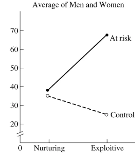
In addition to the three-way interaction there are three main effects to look at, one for each factor. To look at the gender main effect, for instance, just take the average of the scores for all of the men and compare it to the average of all of the women. If you have the cell means handy and the design is balanced, you can average all of the cell means involving men and then all of the cell means involving women. In Table 22.1, you can average the four cell means for the men (40, 28, 36, 48) to get 38 (alternatively, you could use the row means in the extreme right column and average 34 and 42 to get the same result). The aver-age for the women (30, 22, 40, 88) is 45. The means for the other main effects have already been included in Table 22.1. Looking at the bottom row you can see that the mean for the nurturing experimenter is 36.5 as compared to 46.5 for the exploitive one. In the extreme right column you’ll find that the mean for the control subjects is 30, as compared to 53 for the at-risk subjects.
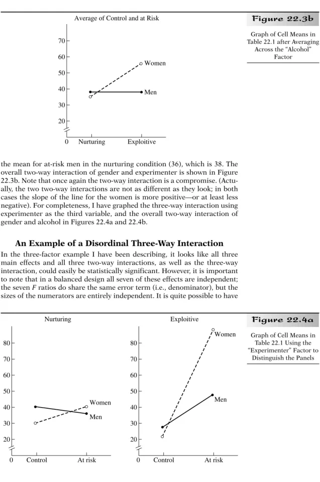
Two-Way Interactions in Three-Way ANOVAs
Further complicating the way ANOVA is that, in addition to the three-way interaction and the three main effects, there are three two-three-way inter-actions to consider. In terms of our example there are the gender by experimenter, gender by alcohol, and experimenter by alcohol interactions. We will look at the last of these first. Before graphing a two-way interaction in a three-factor design, you have to “collapse” (i.e., average) your scores over the variable that is not involved in the two-way interaction. To graph the alco-hol by experimenter (A ×B) interaction you need to average the men with the women for each combination of alcohol and experimenter levels (i.e., each cell of the A ×Bmatrix). These means have also been included in Table 22.1. The graph of these cell means is shown in Figure 22.2. If you compare this overall two-way interaction with the two-way interactions for the men and women separately (see Figure 22.1), you will see that the overall inter-action looks like an average of the two separate interinter-actions; the amount of interaction seen in Figure 22.2 is midway between the amount of interaction for the men and that amount for the women. Does it make sense to average the interactions for the two genders into one overall interaction? It does if they are not very different. How different is too different? The size of the three-way interaction tells us how different these two two-way interactions are. A statistically significant three-way interaction suggests that we should be cautious in interpreting any of the two-way interactions. Just as a signif-icant two-way interaction tells us to look carefully at, and possible test, the
70 60 50 40 30 20 Nurturing 0 Exploitive Control At risk Average of Men and Women
Graph of Cell Means in Table 22.1 after Averaging
Across Gender
Figure 22.2
simple main effects (rather than the overall main effects), a significant three-way interaction suggests that we focus on the simple interaction effects—the two-way interactions at each level of the third variable (which of the three independent variables is treated as the “third” variable is a matter of con-venience). Even if the three-way interaction falls somewhat short of signifi-cance, I would recommend caution in interpreting the two-way interactions and the main effects, as well, whenever the simple interaction effects look completely different and, perhaps, show opposite patterns.
So far I have been focusing on the two-way interaction of alcohol and experimenter in our example, but this choice is somewhat arbitrary. The two genders are populations that we are likely to have theories about, so it is often meaningful to compare them. However, I can just as easily graph the three-way interaction using “alcohol” as the third factor, as I have done in Figure 22.3a. To graph the overall two-way interaction of gender and exper-imenter, you can go back to Table 22.1 and average across the alcohol factor. For instance, the mean for men in the nurturing condition is found by aver-aging the mean for control group men in the nurturing condition (40) with
80 70 60 50 40 30 20 Nurturing 0 Exploitive Women Men Control 80 70 60 50 40 30 20 Nurturing 0 Exploitive Women Men At Risk
Graph of Cell Means in Table 22.1 Using the
“Alcohol” Factor to Distinguish the Panels
Section A
• Conceptual Foundation693
Figure 22.3b
70 60 50 40 30 20 Nurturing 0 Exploitive Women Men Average of Control and at RiskGraph of Cell Means in Table 22.1 after Averaging
Across the “Alcohol” Factor
the mean for at-risk men in the nurturing condition (36), which is 38. The overall two-way interaction of gender and experimenter is shown in Figure 22.3b. Note that once again the two-way interaction is a compromise. (Actu-ally, the two two-way interactions are not as different as they look; in both cases the slope of the line for the women is more positive—or at least less negative). For completeness, I have graphed the three-way interaction using experimenter as the third variable, and the overall two-way interaction of gender and alcohol in Figures 22.4a and 22.4b.
An Example of a Disordinal Three-Way Interaction
In the three-factor example I have been describing, it looks like all three main effects and all three two-way interactions, as well as the three-way interaction, could easily be statistically significant. However, it is important to note that in a balanced design all seven of these effects are independent; the seven Fratios do share the same error term (i.e., denominator), but the sizes of the numerators are entirely independent. It is quite possible to haveFigure 22.4a
80 70 60 50 40 30 20 Control 0 At risk Women Men Nurturing 80 70 60 50 40 30 20 Control 0 At risk Women Men ExploitiveGraph of Cell Means in Table 22.1 Using the “Experimenter” Factor to
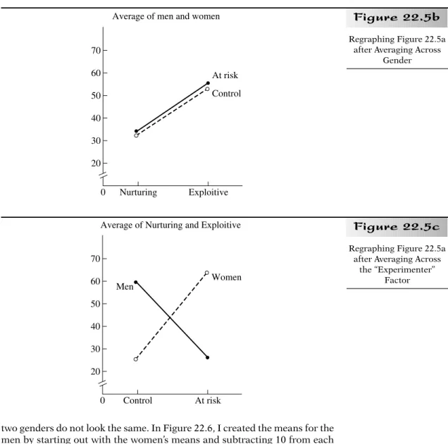
a large three-way interaction while all of the other effects are quite small. By changing the means only for the men in our example, I will illustrate a large, disordinal interaction that obliterates two of the two-way interactions and two of the main effects. You can see in Figure 22.5a that this new three-way interaction is caused by a reversal of the alcohol by experimenter interaction from one gender to the other. In Figure 22.5b, you can see that the overall interaction of alcohol by gender is now zero (the lines are parallel); the gen-der by experimenter interaction is also zero (not shown). On the other hand, the large gender by alcohol interaction very nearly obliterates the main effects of both gender and alcohol (see Figure 22.5c). The main effect of experimenter is, however, large, as can be seen in Figure 22.5b.
An Example in which the Three-Way
Interaction Equals Zero
Finally, I will change the means for the men once more to create an example in which the three-way interaction is zero, even though the graphs for the
70 60 50 40 30 20 Control 0 At risk Women Men Average of Nurturing and Exploitive
Graph of Cell Means in Table 22.1 after Averaging Across the “Experimenter”
Factor
Figure 22.4b
80 70 60 50 40 30 20 Nurturing 0 Expoitive Control At risk Women 80 70 60 50 40 30 20 Nurturing 0 Expoitive Control At risk MenRearranging the Cell Means of Table 22.1 to
Depict a Disordinal 3-Way Interaction
two genders do not look the same. In Figure 22.6, I created the means for the men by starting out with the women’s means and subtracting 10 from each (this creates a main effect of gender); then I added 30 only to the men’s means that involved the nurturing condition. The latter change creates a two-way interaction between experimenter and gender, but because it affects both the men/nurturing means equally, it does not produce any three-way interaction. One three-way to see that the three-three-way interaction is zero in Fig-ure 22.6 is to subtract the slopes of the two lines for each gender. For the women the slope of the at-risk line is positive: 88− 40 =48. The slope of the control line is negative: 22 −30 = −8. The difference of the slopes is 48 −(−8) =56. If we do the same for the men, we get slopes of 18 and −38, whose difference is also 56. You may recall that a 2 ×2 interaction has only one df, and can be summarized by a single number, L, that forms the basis of a simple linear contrast. The same is true for a 2 ×2 × 2 interaction or any higher-order interaction in which all of the factors have two levels. Of course, quantifying a three-way interaction gets considerably more complicated when the fac-tors have more than two levels, but it is safe to say that if the two (or more) graphs are exactly the same, there will be no three-way interaction (they will continue to be identical, even if a different factor is chosen to distinguish the
Section A
• Conceptual Foundation695
Figure 22.5b
70 60 50 40 30 20 Nurturing 0 Exploitive At risk Control Average of men and womenRegraphing Figure 22.5a after Averaging Across
Gender
Figure 22.5c
70 60 50 40 30 20 Control 0 At risk Men Women Average of Nurturing and ExploitiveRegraphing Figure 22.5a after Averaging Across
the “Experimenter” Factor
graphs). Bear in mind, however, that even if the graphs do not lookthe same, the three-way interaction will be zero if the amount of two-way interaction is the same for every graph.
Calculating the Three-Way ANOVA
Calculating a three-way independent-groups ANOVA is a simple extension of the method for a two-way independent-groups ANOVA, using the same basic formulas. In particular, there is really nothing new about calculatingMSW(the
error term for all theFratios); it is just the ordinary average of the cell vari-ances when the design is balanced. (It is hard to imagine that anyone would calculate an unbalanced three-way ANOVA with a calculator rather than a computer, so I will not consider that possibility. The analysis of unbalanced designs is described in general in Chapter 18, Section A). Rather than give you all of the cell standard deviations or variances for the example in Table 22.1, I’ll just tell you thatSSWequals 6,400; later I’ll divide this by dfWto obtainMSW.(If
you had all of the raw scores, you would also have the option of obtainingSSW
by calculatingSStotaland subtractingSSbetween-cellsas defined in the following.)
Main Effects
The calculation of the main effects is also the same as in the two-way ANOVA; the SS for a main effect is just the biased variance of the relevant group means multiplied by the total N.Let us say that each of the eight cells in our example contains five subjects, so NTequals 40. Then the SSfor the
experimenter factor (SSexper) is 40 times the biased variance of 36.5 and 46.5
(the nurturing and exploitive means from Table 22.1), which equals 40(25) = 1000 (the shortcut for finding the biased variance of two numbers is to take the square of the difference between them and then divide by 4). Similarly, SSalcohol=40(132.25) =5290, and SSgender=40(12.25) =490.
The Two-Way Interactions
When calculating the two-way ANOVA, the SSfor the two-way interaction is found by subtraction; it is the amount of the SSbetween-cellsthat is left after
sub-80 70 60 50 40 30 20 Nurturing 0 Expoitive Control At risk Women 80 70 60 50 40 30 20 Nurturing 0 Expoitive Control At risk Men
Rearranging the Cell Means of Table 22.1 to Depict a Zero Amount of
Three-Way Interaction
tracting the SSs for the main effects. Similarly, the three-way interaction SS is the amount left over after subtracting the SSs for the main effects and the SSs for all the two-way interactions from the overall SSbetween-cells. However,
finding the SSs for the two-way interactions in a three-way design gets a lit-tle tricky. In addition to the overall SSbetween-cells, we must also calculate some
intermediate “two-way” SSbetweenterms.
To keep track of these I will have to introduce some new subscripts. The overall SSbetween-cellsis based on the variance of all the cell means, so no factors
are “collapsed,” or averaged over. Representing gender as G,alcohol as A,and experimenter as E,the overall SSbetween-cellswill be written as SSGAE.We will
also need to calculate an SSbetweenafter averaging over gender. This is based on
the four means (included in Table 22.1) I used to graph the alcohol by exper-imenter interaction and will be represented by SSAE.Because the design is
balanced, you can take the simple average of the appropriate male cell mean and female cell mean in each case. Note that SSAEis not the SSfor the
alco-hol by experimenter interaction because it also includes the main effects of those two factors. In similar fashion, we need to find SSGAfrom the means
you get after averaging over the experimenter factor and SSGEby averaging
over the alcohol factor. Once we have calculated these four SSbetweenterms, all
of the SSs we need for the three-way ANOVA can be found by subtraction. Let’s begin with the calculation of SSGAE;the biased variance of the eight
cell means is 366.75, so SSGAE=40(366.75) =14,670. The means for SSAEare
35, 25, 38, 68, and their biased variance equals 257.75, so SSAE=10,290. SSGA
is based on the following means: 34, 26, 42, 64, so SSGA=40(200.75) =8,030.
Finally, SSGE,based on means of 38, 38, 35, 55, equals 2,490.
Next we find the SSs for each two-way interaction:
SSA×E=SSAE−SSalcohol−SSexper=10,290 −5,290 −1,000 =4,000 SSG×A=SSGA−SSgender−SSalcohol=8,030 −490 −5,290 =2,250 SSG×E=SSGE−SSgender−SSexper=2,490 −490 −1,000 =1,000
Finally, the SSfor the three-way interaction (SSG×A×E) equals
SSGAE−SSA×E−SSG×A−SSG×E−SSgender−SSalcohol−SSexper =14,670 −4,000 −2,250 −1,000 −490 −5,290 −1,000 =640
Formulas for the General Case
It is traditional to assign the letters A, B,and, C to the three independent variables in the general case; variables D, E,and so forth, can then be added to represent a four-way, five-way, or higher ANOVA. I’ll assume that the fol-lowing components have already been calculated using Formula 14.3 applied to the appropriate means: SSA, SSB, SSC, SSAB, SSAC, SSBC, SSABC.In
addition, I’ll assume that SSWhas also been calculated, either by averaging
the cell variances and multiplying by dfWor by subtracting SSABCfrom SStotal.
The remaining SScomponents are found by Formula 22.1:
a. SSA×B=SSAB−SSA−SSB Formula 22.1
b. SSA×C=SSAC−SSA−SSC
c. SSB×C=SSBC−SSB−SSC
d. SSA×B×C=SSABC−SSA×B−SSB×C−SSA×C−SSA−SSB−SSC
At the end of the analysis, SStotal(whether or not it has been calculated
separately) has been divided into eight components: SSA, SSB, SSC,the four
interactions listed in Formula 22.1, and SSW.Each of these is divided by its
corresponding df to form a variance estimate, MS.Using ato represent the
number of levels of the Afactor, bfor the Bfactor, cfor the Cfactor, and n for the number of subjects in each cell, the formulas for the df components are as follows: a. dfA=a−1 Formula 22.2 b. dfB=b−1 c. dfC=c−1 d. dfA×B=(a−1)(b−1) e. dfA×C=(a−1)(c−1) f. dfB×C=(b−1)(c−1) g. dfA×B×C=(a−1)(b−1)(c−1) h. dfW=abc(n−1)
Completing the Analysis for the Example
Because each factor in the example has only two levels, all of the numerator df’s are equal to 1, which means that all of the MSterms are equal to their corresponding SSterms—except, of course, for the error term. The df for the error term (i.e., dfW) equals the number of cells (abc) times one less than the
number of subjects per cell (this gives the same value as NTminus the
num-ber of cells); in this case dfW= 8(4) = 32. MSW= SSW/dfW; therefore, MSW=
6400/32 = 200. (Reminder: I gave the value of SSW to you to reduce the
amount of calculation.)
Now we can complete the three-way ANOVA by calculating all of the possible Fratios and testing each for statistical significance:
Fgender= = =2.45 Falcohol= = =26.45 Fexper= = =5 FA×E= = =20 FG×A= = =11.35 FG×E= = =5 FG×A×E= = =3.2
Because the df happens to be 1 for all of the numerator terms, the critical F for all seven tests is F.05(1,32), which is equal (approximately) to 4.15. Except
for the main effect of gender, and the three-way interaction, all of the Fratios exceed the critical value (4.15) and are therefore significant at the .05 level.
Follow-Up Tests for the Three-Way ANOVA
Decisions concerning follow-up comparisons for a factorial ANOVA are made in a top-down fashion. First, one checks the highest-order interaction
640 200 MSG×A×E MS W 1000 200 MSG×E MS W 2,250 200 MSG×A MS W 4,000 200 MSA×E MS W 1,000 200 MSexper MS W 5,290 200 MSalcohol MS W 490 200 MSgender MS W
for significance; in a three-way ANOVA it is the three-way interaction. (Two-way interactions are the simplest possible interactions and are called first-order interactions; three-way interactions are known as second-order interactions, etc.) If the highest interaction is significant, the post hoc tests focus on the various simple effects or interaction contrasts, followed by appropriate cell-to-cell comparisons. In a three-way ANOVA in which the three-way interaction is not significant, as in the present example, attention turns to the three two-way interactions. Although all of the two-way interac-tions are significant in our example, the alcohol by experimenter interaction is the easiest to interpret because it replicates previous results.
It would be appropriate to follow up the significant alcohol by experi-menter interaction with four ttests (e.g., one of the relevant t tests would determine whether at-risk subjects differ significantly from controls in the exploitive condition). Given the disordinal nature of the interaction (see Fig-ure 22.2), it is likely that the main effects would simply be ignored. A similar approach would be taken to the two other significant two-way interactions. Thus, all three main effects would be regarded with caution. Note that because all of the factors are dichotomous, there would be no follow-up tests to perform on significant main effects, even if none of the interactions were significant. With more than two levels for some or all of the factors, it becomes possible to test partial interactions, and significant main effects for factors not involved in significant interactions can be followed by pairwise or complex comparisons, as described in Chapter 14, Section C. I will illus-trate some of the complex planned and post hoc comparisons for the three-way design in Section B.
Types of Three-Way Designs
Cases involving significant three-way interactions and factors with more than two levels will be considered in the context of mixed designs in Section B. However, before we turn to mixed designs, let us look at some of the typ-ical situations in which three-way designs with no repeated measures arise. One situation involves three experimental manipulations for which repeated measures are not feasible. For instance, subjects perform a repetitive task in one of two conditions: They are told that their performance is being meas-ured or that it is not. In each condition half of the subjects are told that per-formance on the task is related to intelligence, and the other half are told that it is not. Finally, within each of the four groups just described, half the subjects are treated respectfully and half are treated rudely. The work output of each subject can then be analyzed by a 2 ×2 ×2 ANOVA.
Another possibility involves three grouping variables, each of which involves selecting subjects whose group is already determined. For instance, a group of people who exercise regularly and an equal-sized group of those who don’t are divided into those high and those relatively low on self-esteem (by a median split). If there are equal numbers of men and women in each of the four cells, we have a balanced 2 ×2 ×2 design. More commonly one or two of the variables involve experimental manipulations and two or one involve grouping variables. The example calculated earlier in this section involved two grouping variables (gender and having an alcohol-dependent parent or not) and one experimental variable (nurturing vs. exploitive experimenter).
To devise an interesting example with two experimental manipulations and one grouping variable, start with two experimental factors that are expected to interact (e.g., one factor is whether or not the subjects are told that performance on the experimental task is related to intelligence, and the other factor is whether or not the group of subjects run together will know
each other’s final scores). Then, add a grouping variable by comparing sub-jects who are either high or low on self-esteem, need for achievement, or some other relevant aspect of personality. If the two-way interaction differs significantly between the two groups of subjects, the three-way interaction will be significant.
The Two-Way RM ANOVA
One added benefit of learning how to calculate a three-way ANOVA is that you now know how to calculate a two-way ANOVA in which both factors involve repeated measures. In Chapter 15, I showed you that the SS compo-nents of a one-way RM design are calculated as though the design were a two-way independent-groups ANOVA with no within-cell variability. Simi-larly, a two-way RM ANOVA is calculated just as shown in the preceding for the three-way independent-groups ANOVA, with the following modifica-tions: (1) One of the three factors is the subjects factor—each subject repre-sents a different level of the subjects factor, (2) the main effect of subjects is not tested, and there is no MSWerror term, (3) each of the two main effects
that istested uses the interaction of that factor with the subjects factor as the error term, and (4) the interaction of the two factors of interest is tested by using as the error term the interaction of all three factors (i.e., including the subjects factor). If one RM factor is labeled Qand the other factor, R,and we use Sto represent the subjects factor, the equations for the three Fratios can be written as follows:
FQ= , FR= FQ×R=
Higher-Order ANOVA
This text will not cover factorial designs of higher order than the three-way ANOVA. Although higher-order ANOVAs can be difficult to interpret, no new principles are introduced. The four-way ANOVA produces 15 different F ratios to test: four main effects, 6 two-way interactions, 4 three-way interac-tions, and 1 four-way interaction. Testing each of these 15 effects at the .05 level raises serious concerns about the increased risk of Type I errors. Usu-ally, all of the Fratios are not tested; specific hypotheses should guide the selection of particular effects to test. Of course, the potential for an inflated rate of Type I errors only increases as factors are added. In general, an N-way ANOVA produces 2N−1 Fratios that can be tested for significance.
In the next section I will delve into more complex varieties of the three-way ANOVA—in particular those that include repeated measures on one or two of the factors.
1. To display the cell means of a three-way factorial design, it is convenient to create two-way graphs for each level of the third variable and place these graphs side by side (you have to decide which of the three ables will distinguish the graphs and which of the two remaining vari-ables will be placed along the Xaxis of each graph). Each two-way graph depicts a simple interaction effect; if the simple interaction effects are significantly different from each other, the three-way interaction will be significant.
2. Three-way interactions can occur in a variety of ways. The interaction of two of the factors can be strong at one level of the third factor and close
MSQ×R MX Q×R×S MSR MS R×S MSQ MS Q×S
A
SUMMARY
to zero at a different level (or even stronger at a different level). The direction of the two-way interaction can reverse from one level of the third variable to another. Also, a three-way interaction can arise when all of the cell means are similar except for one.
3. The main effects of the three-way ANOVA are based on the means at each level of one of the factors, averaging across the other two. A two-way interaction is the average of the separate two-two-way interactions (simple interaction effects) at each level of the third factor. A two-way interaction is based on a two-way table of means created by averaging across the third factor.
4. The error term for the three-way ANOVA, MSW,is a simple extension of
the error term for a two-way ANOVA; in a balanced design, it is the sim-ple average of all of the cell variances. All of the SSbetweencomponents are
found by Formula 14.3, or by subtraction using Formula 22.1. There are seven Fratios that can be tested for significance: the three main effects, three two-way interactions, and the three-way interaction.
5. Averaging simple interaction effects together to create a two-way inter-action is reasonable only if these effects do not differ significantly. If they do differ, follow-up tests usually focus on the simple interaction effects themselves or particular 2 ×2 interaction contrasts. If the three-way interaction is not significant, but a two-three-way interaction is, the sig-nificant two-way interaction is explored as in a two-way ANOVA—with simple main effects or interaction contrasts. Also, when the three-way interaction is not significant, any significant main effect can be followed up in the usual way if that variable is not involved in a significant two-way interaction.
6. All three factors in a three-way ANOVA can be grouping variables (i.e., based on intact groups), but this is rare. It is more common to have just one grouping variable and compare the interaction of two experimental factors among various subgroups of the population. Of course, all three factors can involve experimental manipulations.
7. The two-way ANOVA in which both factors involve repeated measures is analyzed as a three-way ANOVA, with the different subjects serving as the levels of the third factor. The error term for each RM factor is the interaction of that factor with the subject factor; the error term for the interaction of the two RM factors is the three-way interaction.
8. In an N-way factorial ANOVA, there are 2N−1 Fratios that can be tested.
The two-way interaction is called a first-order interaction, the three-way is a second-order interaction, and so forth.
Section A
• Conceptual Foundation701
1. Imagine an experiment in which each sub-ject is required to use his or her memories to create one emotion: either happiness, sad-ness, anger, or fear. Within each emotion group, half of the subjects participate in a relaxation exercise just before the emotion condition, and half do not. Finally, half the subjects in each emotion/relaxation condi-tion are run in a dark, sound-proof chamber, and the other half are run in a normally lit room. The dependent variable is the subject’s
systolic blood pressure when the subject sig-nals that the emotion is fully present. The design is balanced, with a total of 128 sub-jects. The results of the three-way ANOVA for this hypothetical experiment are as follows: SSemotion =223.1, SSrelax =64.4, SSdark =31.6, SSemo×rel=167.3, SSemo×dark=51.5; SSrel×dark=
127.3, and SSemo×rel×dark=77.2. The total sum
of squares is 2,344.
a. Calculate the seven Fratios, and test each for significance.
b. Calculate partial eta squared for each of the three main effects (use Formula 14.9). Are any of these effects at least moderate in size?
2. In this exercise there are 20 subjects in each cell of a 3 ×3 ×2 design. The levels of the first factor (location) are urban, suburban, and rural. The levels of the second factor are no siblings, one or two siblings, and more than two siblings. The third factor has only two levels: presently married and not presently married. The dependent variable is the num-ber of close friends that each subject reports having. The cell means are as follows:
a. Given that SSWequals 1,094, complete the
three-way ANOVA, and present your results in a summary table.
b. Draw a graph of the means for Location × Number of Siblings (averaging across mar-ital status). Describe the nature of the interaction.
c. Using the means from part b, test the sim-ple effect of number of siblings at each location.
3. Seventy-two patients with agoraphobia are randomly assigned to one of four drug condi-tions: SSRI (e.g., Prozac), tricyclic antidepres-sant (e.g., Elavil), antianxiety (e.g., Xanax), or a placebo (offered as a new drug for agora-phobia). Within each drug condition, a third of the patients are randomly assigned to each of three types of psychotherapy: psychody-namic, cognitive/behavioral, and group. The subjects are assigned so that half the subjects in each drug/therapy group are also de-pressed, and half are not. After 6 months of treatment, the severity of agoraphobia is measured for each subject (30 is the maxi-mum possible phobia score); the cell means (n=3) are as follows:
a. Given that SSW equals 131, complete the
three-way ANOVA, and present your results in a summary table.
b. Draw a graph of the cell means, with sep-arate panels for depressed and not depressed. Describe the nature of the therapy × drug interaction in each panel. Does there appear to be a three-way inter-action? Explain.
c. Given your results in part a, describe a set of follow-up tests that would be justifi-able.
d. Optional: Test the 2 × 2 × 2 interaction contrast that results from deleting Group therapy and the SSRI and placebo condi-tions from the analysis (extend the tech-niques of Chapter 13, Section B, and Chapter 14, Section C).
4. An industrial psychologist is studying the relation between motivation and productiv-ity. Subjects are told to perform as many repetitions of a given clerical task as they can in a 1-hour period. The dependent vari-able is the number of tasks correctly per-formed. Sixteen subjects participated in the experiment for credit toward a requirement of their introductory psychology course (credit group). Another 16 subjects were recruited from other classes and paid $10 for the hour (money group). All subjects performed a small set of similar clerical tasks as practice before the main study; in each group (credit or money) half the sub-jects (selected randomly) were told they had performed unusually well on the practice trials (positive feedback), and half were told they had performed poorly (negative feed-back). Finally, within each of the four groups created by the manipulations just described, half of the subjects (at random) were told that performing the tasks quickly and accurately was correlated with other important job skills (self motivation), whereas the other half were told that good performance would help the experiment (other motivation). The data appear in the following table:
Urban Suburban Rural
No Siblings Married 1.9 3.1 2.0 Not Married 4.7 5.7 3.5 1 or 2 Siblings Married 2.3 3.0 3.3 Not Married 4.5 5.3 4.6 2 or more Siblings Married 3.2 4.5 2.9 Not Married 3.9 6.2 4.6
SSRI Tricyclic Antianxiety Placebo Psychodynamic Not Depressed 10 11.5 19.0 22.0 Depressed 8.7 8.7 14.5 19.0 Cog/Behav Not Depressed 9.5 11.0 12.0 17.0 Depressed 10.3 14.0 10.0 16.5 Group Not Depressed 11.6 12.6 19.3 13.0 Depressed 9.7 12.0 17.0 11.0
a. Perform a three-way ANOVA on the data. Test all seven Fratios for significance, and present your results in a summary table. b. Use graphs of the cell means to help you
describe the pattern underlying each effect that was significant in part a. c. Based on the results in part a, what post
hoc tests would be justified?
5. Imagine that subjects are matched in blocks of three based on height, weight, and other physical characteristics; six blocks are formed in this way. Then the subjects in each block are randomly assigned to three
differ-ent weight-loss programs. Subjects are meas-ured before the diet, at the end of the diet program, 3 months later, and 6 months later. The results of the two-way RM ANOVA for this hypothetical experiment are given in terms of the SS components, as follows: SSdiet = 403.1, SStime = 316.8, SSdiet×time = 52, SSdiet×S=295.7, SStime×S=174.1, and SSdiet×time×S
=230.
a. Calculate the three Fratios, and test each for significance.
b. Find the conservatively adjusted critical F for each test. Will any of your conclusions be affected if you do not assume that sphericity exists in the population? 6. A psychologist wants to know how both the
affective valence (happy vs. sad vs. neutral) and the imageability (low, medium, high) of words affect their recall. A list of 90 words is prepared with 10 words from each combina-tion of factors (e.g., happy, low imagery: pro-motion; sad, high imagery: cemetery) randomly mixed together. The number of words recalled in each category by each of the six subjects in the study is given in the following table:
a. Perform a two-way RM ANOVA on the data. Test the three Fratios for significance, and present your results in a summary table. b. Find the conservatively adjusted critical F
for each test. Will any of your conclusions be affected if you do not assume that sphericity exists in the population?
c. Draw a graph of the cell means, and describe any trend toward an interaction that you can see.
d. Based on the variables in this exercise, and the results in part a, what post hoc tests would be justified and mean-ingful?
Section B
• Basic Statistical Procedures703
CREDITSUBJECTS PAIDSUBJECTS
Positive Negative Positive Negative
Feedback Feedback Feedback Feedback
Self 22 12 21 25 25 15 17 23 26 12 15 30 30 10 21 26 Other 11 20 33 21 18 23 29 22 12 21 35 19 14 26 29 17 SAD NEUTRAL HAPPY
Subject No. Low Medium High Low Medium High Low Medium High
1 5 6 9 2 5 6 3 4 8 2 2 5 7 3 6 6 5 5 6 3 5 7 5 2 4 5 4 3 7 4 3 6 5 3 5 6 4 4 5 5 4 9 8 4 7 7 4 5 9 6 3 5 7 4 5 6 6 4 4
An important way in which one three-factor design can differ from another is the number of factors that involve repeated measures (or matching). The design in which none of the factors involve repeated measures was covered in Section A. The design in which all three factors are RM factors will not be covered in this text; however, the three-way RM design is a straightforward extension of the two-way RM design described at the end of Section A. This section will focus on three-way designs with either one or two RM factors (i.e., mixed designs), and it will also elaborate on the general principles of dealing with three-way ANOVAs, as introduced in Section A, and consider
B
BASIC
STATISTICAL
PROCEDIRES
the complexities of interactions and post hoc tests when the factors have more than two levels each.
One RM Factor
I will begin with a three-factor design in which there are repeated measures on only one of the factors. The ANOVA for this design is not much more complicated than the two-way mixed ANOVA described in the previous chapter—for instance, there are only two different error terms. Such designs arise frequently in psychological research. One simple way to arrive at such a design is to start with a two-way ANOVA with no repeated measures. For instance, patients with two different types of anxiety disorders (generalized anxiety vs. specific phobias) are treated with two different forms of psy-chotherapy (psychodynamic vs. behavioral). The third factor is added by measuring the patients’ anxiety at several points in time (e.g., beginning of therapy, end of therapy, several months after therapy has stopped); I will refer to this factor simply as time.
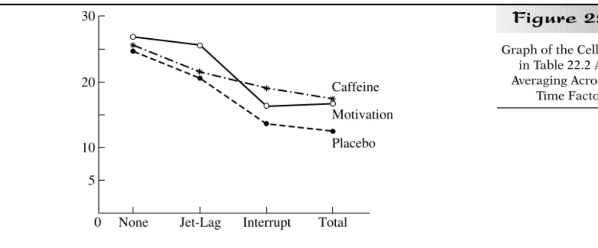
To illustrate the analysis of this type of design I will take the two-way ANOVA from Section B of Chapter 14 and add time as an RM factor. You may recall that that example involved four levels of sleep deprivation and three levels of stimulation. Performance was measured only once—after 4 days in the sleep lab. Now imagine that performance on the simulated truck driving task is measured three times: after 2, 4, and 6 days in the sleep lab. The raw data for the three-factor study are given in Table 22.2, along with the various means we will need to graph and analyze the results; note that the data for Day 4 are identical to the data for the corresponding two-way ANOVA in Chapter 14. To see what we may expect from the results of a three-way ANOVA on these data, the cell means have been graphed so that we can look at the sleep by stimulation interaction at each time period (see Figure 22.7).
You can see from Figure 22.7 that the sleep × stimulation interaction, which was not quite significant for Day 4 alone (see Chapter 14, section B), increases over time, perhaps enough so as to produce a three-way interac-tion. We can also see that the main effects of stimulation and sleep, signifi-cant at Day 4, are likely to be signifisignifi-cant in the three-way analysis. The general decrease in scores from Day 2 to Day 4 to Day 6 is also likely to yield a significant main effect for time. Without regraphing the data, it is hard to see whether the interactions of time with either sleep or stimulation are large or small. However, because these interactions are less interesting in the context of this experiment, I won’t bother to present the two other possible sets of graphs.
To present general formulas for analyzing the kind of experiment shown in Table 22.2, I will adopt the following notation. The two between-subject factors will be labeled A and B. Of course, it is arbitrary which factor is called Aand which B;in this example the sleep deprivation factor will be A, and the stimulation factor will be B.The lowercase letters aand bwill stand for the number of levels of their corresponding factors—in this case, 4 and 3, respectively. The within-subject factor will be labeled R,and its number of levels, c,to be consistent with previous chapters.
Let us begin with the simplest SScomponents: SStotal, and the SSs for
the numerators of each main effect. SStotalis based on the total number of
observations, NT, which for any balanced three-way factorial ANOVA is
equal to abcn,where nis the number of different subjects in each cell of the A ×Btable. So, NT=4 3 3 5 =180. The biased variance obtained by
P
LA CEBOM
O TIV A TIONC
AFFEINE Subject Subject Subject R o w Da y 2 D a y 4 D a y 6 Means Da y 2 D a y 4 D a y 6 Means Da y 2 D a y 4 D a y 6 Means Means 26 24 24 24.67 29 28 26 27.67 29 26 26 27.0 30 29 25 28.0 26 23 23 24.0 24 22 23 23.0 None 29 28 27 28.0 23 24 25 24.0 23 20 17 20.0 23 20 20 21.0 29 30 27 28.67 31 30 30 30.33 21 20 20 20.33 35 33 22 30.0 29 27 25 27.0 AB means 25.8 24.2 23.2 24.4 28.4 27.6 24.6 26.87 27.2 25.0 24.2 25.47 25.58 24 22 17 21 27 26 33 28.67 24 25 20 23 20 18 15 17.67 29 30 17 25.33 30 27 24 27.0 Jet Lag 15 16 13 14.67 34 32 25 30.33 30 31 25 28.67 27 25 19 23.67 23 20 18 20.33 25 24 17 22.0 28 27 22 25.67 25 23 20 22.67 23 21 22 22.0 AB means 22.8 21.6 17.2 20.53 27.6 26.2 22.6 25.46 26.4 25.6 21.6 24.53 23.51 17 16 9 14.0 25 16 10 17.0 23 23 20 22.0 19 19 6 14.67 21 13 9 14.33 29 28 23 26.67 Interr upt 22 20 11 17.67 19 12 8 1 3.0 2 8 2 6 2 3 25.67 11 11 7 9.67 25 18 12 18.33 20 17 12 16.33 15 14 10 13.0 24 19 14 19.0 21 19 17 19.0 AB means 16.8 16.0 8.6 13.8 22.8 15.6 10.6 16.33 24.2 22.6 19.0 21.93 17.35 16 14 5 11.67 24 15 14 17.67 25 23 18 22.0 18 17 6 13.67 19 11 8 12.67 16 16 14 15.33 T otal 20 18 10 16.0 20 11 15 15.33 19 18 12 16.33 14 12 7 11.0 27 19 17 21.0 27 26 21 24.67 11 10 7 9.33 26 17 10 17.67 26 24 21 23.67 AB means 15.8 14.2 7.0 12.33 23.2 14.6 12.8 16.87 22.6 21.4 17.2 20.4 16.53 Column means 20.3 19.0 14.0 17.77 25.5 21.0 17.65 21.38 25.1 23.65 20.5 23.08T
able 22.2
on the means for the four sleep deprivation levels, which can be found in the rightmost column of the table, labeled “row means.” SSBis based on the
means for the three stimulation levels, which are found where the bottom row of the table (Column Means), intersects the columns labeled “Subject Means” (these are averaged over the three days, as well as the sleep levels). The means for the three different days are not in the table but can be found by averaging the three Column Means for Day 2, the three for Day 4, and similarly for Day 6. The SSs for the main effects are as follows:
SSA= σ2(25.58, 23.51, 17.35, 16.53) 180 =15.08 180 =2,714.4.
SSB= σ2(17.77, 21.38, 23.08) 180 =4.902 180 =882.36.
SSR= σ2(23.63, 21.22, 17.38) =6.622 180 =1,192.0
As in Section A, we will need the SSbased on the cell means, SSABR,and
the SSs for each two-way table of means: SSAB, SSAR,and SSBR.In addition,
because one factor has repeated measures we will also need to find the means for each subject (averaging their scores for Day 2, Day 4, and Day 6) and the SSbased on those means, SSbetween-subjects.
30 25 20 15 10 7 None Jet-Lag 0 Interrupt Total Placebo Caffeine Day 2 Motivation 30 25 20 15 10 7 None Jet-Lag 0 Interrupt Total Placebo Caffeine Day 4 Motivation 30 25 20 15 10 7 None Jet-Lag 0 Interrupt Total Placebo Caffeine Day 6 Motivation
Graph of the Cell Means in Table 22.2
The cell means we need for SSABRare given in Table 22.2, under Day 2,
Day 4, and Day 6, in each of the rows labeled ABMeans; there are 36 of them (a b c). The biased variance of these cell means is 30.746, so SSABR=
30.746 180 =5,534.28. The means for SSABare found by averaging across
the 3 days for each combination of sleep and stimulation levels and are found in the rows for AB Means under “Subject Means.” The biased variance of these 12 (i.e., a b) means equals 22.078, so SSAB=3,974. The nine means
for SSBRare the column means of Table 22.2, except for the columns labeled
“Subject Means.” SSBR = σ2(20.3, 19.0, 14.0, 25.5, 21.0, 17.65, 25.1, 23.65,
20.5) 180 =2,169.14. Unfortunately, there was no convenient place in Table 22.2 to put the means for SSAR.They are found by averaging the (AB) means
for each day and level of sleep deprivation over the three stimulation levels. SSAR= σ2(27.13, 25.6, 24, 25.6, 24.47, 20.47, 21.27, 18.07, 12.73, 20.53, 16.73,
12.33) 180 =4,066.6. Finally, we need to calculate SSbetween-subjectsfor the 60
(a b n) subject means found in Table 22.2 under “Subject Means” (ignor-ing the entries in the rows labeled ABMeans and Column Means, of course).
SSbetween-subjects=32.22 180 =5,799.6.
Now we can get the rest of the SScomponents we need by subtraction. The SSs for the two-way interactions are found just as in Section A from Formula 22.1a, b, and c (except that factor C has been changed to R):
SSA×B=SSAB−SSA−SSB
SSA×R=SSAR−SSA−SSR
SSB×R=SSBR−SSB−SSR
Plugging in the SSs for the present example, we get SSA×B=3,974 −2,714.4 −882.4 =377.2
SSA×R=4,066.6 −2,714.4 −1,192 =160.2
SSB×R=2,169.14 −882.4 −1,192 =94.74
The three-way interaction is found by subtracting from SSABRthe SSs for
three two-way interactions and the three main effects (Formula 22.1d). SSA×B×R=SSABR−SSA×B−SSA×R−SSB×R−SSA−SSB−SSR
SSA×B×R=5,534.28 −377.2 −160.2 −94.74 −2,714.4 −882.4 −1192 =113.34
As in the two-way mixed design there are two different error terms. One of the error terms involves subject-to-subject variability within each group— or, in the case of the present design, within each cell formed by the two between-group factors. This is the error component you have come to know as SSW,and I will continue to call it that. The total variability from one
sub-ject to another (averaging across the RM factor) is represented by a term we have already calculated: SSbetween-subjects, or SSbet-s, for short. In the one-way
RM ANOVA this source of variability was called the “subjects” factor (SSsub),
or the main effect of “subjects,” and because it did not play a useful role, we ignored it. In the mixed design of the previous chapter it was simply divided between SSgroupsand SSW.Now that we have two between-group factors, that
source of variability can be divided into four components, as follows: SSbet-s=SSA+SSB+SSA×B+SSW
This relation can be expressed more simply as SSbet-s=SSAB+SSW
The error portion, SSW, is found most easily by subtraction:
SSW=SSbet-S−SSAB Formula 22.3
This SSis the basis of the error term that is used for all three of the between-group effects. The other error term involves the variability within subjects. The total variability within subjects, represented by SSwithin-subjects, or SSW-S,
for short, can be found by taking the total SSand subtracting the between-subject variability:
SSW-S=SStotal−SSbet-S Formula 22.4
The within-subject variability can be divided into five components, which include the main effect of the RM factor and all of its interactions:
SSW-S=SSR+SSA×R+SSB×R+SSA×B×R+SSS×R
The last term is the basis for the error term that is used for all of the effects involving the RM factor (it was called SSS×RM in Chapter 16). It is
found conveniently by subtraction:
SSS×R=SSW-S−SSR−SSA×R−SSB×R−SSA×B×R Formula 22.5
We are now ready to get the remaining SScomponents for our example. SSW=SSbet-S−SSAB=5,799.6 −3,974 =1,825.6
SSW-S=SStotal−SSbet-S=7,768.24 −5,799.6 =1,968.64 SSS×R=SSW-S−SSR−SSA×R−SSB×R−SSA×B×R
=1,968.64 −1,192 −160.2 −94.74 −113.34 =408.36
A more tedious but more instructive way to find SSS×Rwould be to find
the subject by RM interaction separately for each of the eight cells of the between-groups (AB) matrix and then add these eight components together. This overall error term is justified only if you can assume that all eight inter-actions would be the same in the entire population. As mentioned in the pre-vious chapter, there is a statistical test (Box’s M criterion) that can be used to give some indication of whether this assumption is reasonable.
Now that we have divided SStotalinto all of its components, we need to
do the same for the degrees of freedom. This division, along with all of the df formulas, is shown in the degrees of freedom tree in Figure 22.8.
The df’s we will need to complete the ANOVA are based on the following formula: a. dfA=a−1 Formula 22.6 b. dfB=b−1 c. dfA×B=(a−1)(b−1) d. dfR=c−1 e. dfA×R=(a−1)(c−1) f. dfB×R=(b−1)(c−1) g. dfA×B×R=(a−1)(b−1)(c−1) h. dfW=ab(n−1) i. dfS×R=dfWdfR=ab(n−1)(c−1)
For the present example, dfA=4 −1 =3 dfB=3 −1 =2 dfA×B=3 2 =6 dfR=3 −1 =2 dfA×R=3 2 =6 dfB×R=2 2 =4 dfA×B×R=3 2 2 =12 dfW=4 3 (5 −1) =48 dfS×R=dfWdfR=48 2 =96
Note that the sum of all the df’s is 179, which equals dftotal(NT−1 =abcn−1 =
180 −1).
The next step is to divide each SSby its df to obtain the corresponding MS.The results of this step are shown in Table 22.3 along with the F ratios and their pvalues. The seven F ratios were formed according to Formula 22.7:
Section B
• Basic Statistical Procedures709
Figure 22.8
df total [abcn–1] df groups [ab–1] df W [ab(n–1)] df between-subjects [abn–1] df R [c–1] df S × R [ab(n–1)(c–1)] df A [a–1] df B [b–1] df A × B [(a–1)(b–1)] df A × R [(a–1)(c–1)] df B × R [(b–1)(c–1)] df A × B × R [(a–1)(b–1)(c–1)] df within-subjects [abn(c–1)]Degrees of Freedom Tree for Three-Way ANOVA with Repeated Measures
on One Factor Source SS df MS F p Between-subjects 5,799.6 59 Sleep deprivation 2714.4 3 904.8 23.8 <.001 Stimulation 882.4 2 441.2 11.6 <.001 Sleep ×Stim 375.8 6 62.63 1.65 >.05 Within-groups 1825.6 48 38.03 Within-subjects 1,968.64 120 Time 1192 2 596 140.2 <.001 Sleep ×Time 160.2 6 26.7 6.28 <.001 Stim ×Time 94.74 4 23.7 5.58 <.001
Sleep ×Stim ×Time 114.74 12 9.56 2.25 <.05
Subject ×Time 408.36 96 4.25
Note:The errors that you get from rounding off the means before applying Formula 14.3 are compounded in a complex design. If you retain more digits after the decimal place than I did in the various group and cell means or use raw-score formulas or analyze the data by computer, your Fratios will differ by a few tenths of a point from those in Table 22.3 (fortunately, your conclusions should be the same). If you are going to present your findings to others, regardless of the purpose, I strongly recommend that you use statistical software, and in particular a program or package that is quite popular (so that there is a good chance that its bugs have already been eliminated, at least for basic procedures, such as those in this text).
a. FA= Formula 22.7 b. FB= c. FA×B= d. FR= e. FA×R= f. FB×R= g. FA×B×R=
Interpreting the Results
Although the three-way interaction is significant, the ordering of most of the effects is consistent enough that the main effects are interpretable. The sig-nificant main effect of sleep is due to a general decline in performance across the four levels, with “no deprivation” producing the least deficit and “total deprivation” the most, as would be expected. It is also no surprise that overall performance significantly declines with increased time in the sleep lab. The significant stimulation main effect seems to be due mainly to the consistently lower performance of the placebo group rather than the fairly small difference between caffeine and reward.
In Figure 22.9, I have graphed the sleep by stimulation interaction, by averaging the three panels of Figure 22.7. Although the interaction looks like it might be significant, we know from Table 22.3 that it is not. Remember that the error term for testing this interaction is based on subject-to-subject variability within each cell and does not benefit from the added power of repeated measures. The other two interactions use MSS×RMas their error
term and therefore do gain the extra power usually conferred by repeated measures. Of course, even if the sleep by stimulation interaction were sig-nificant, its interpretation would be qualified by the significance of the three-way interaction. The significant three-way interaction tells us to be cautious in our interpretation of the other six Fratios and suggests that we look at simple interaction effects.
There are three ways to look at simple interaction effects in a three-way ANOVA (depending on which factor is looked at one level at a time), but the most interesting two-way interaction for the present example is sleep depri-vation by stimulation, so we will look at that interaction at each level of the time factor. The results have already been graphed this way in Figure 22.7. It is easy to see that the three-way interaction in this study is due to the pro-gressive increase in the sleep by stimulation interaction over time.
MSA×B×R MS S×R MSB×R MS S×R MSA×R MS S×R MSR MS S×R MSA×B MS W MSB MS W MSA MS W
Assumptions
The sphericity tests and adjustments you learned in Chapters 15 and 16 are easily extended to apply to this design as well. Box’s M criterion can be used to test that the covariances for each pair of RM levels are the same (in the population) for every combination of the two between-group factors. If M is not significant, the interactions can be pooled across all the cells of the two-way between-groups part of the design and then tested for sphericity with Mauchley’s W. If you cannot perform these tests (or do not trust them), you can use the modified univariate approach as described in Chapter 15. A fac-torial MANOVA is also an option (see section C). The df’s and plevels for the within-subjects effects in Table 22.3 were based on the assumption of sphericity. Fortunately, the effects are so large that even using the most con-servative adjustment of the df’s (i.e., lower-bound epsilon), all of the effects remain significant at the .05 level (although the three-way interaction is just at the borderline with p=.05).
Follow-up Comparisons: Simple Interaction Effects
To test the significance of the simple interaction effects just discussed, the appropriate error term is MSwithin-cell, as defined in section C of Chapter 16,
rather than MSWfrom the overall analysis. This entails adding SSWto SSS×R
and dividing by the sum of dfWand dfS×R. Thus, MSwithin-cellequals (1,827 +
407)/(48 +96) =2,234/144 =15.5. However, given the small sample sizes in our example, it would be even safer (with respect to controlling Type I errors) to test the two-way interaction in each simple interaction effect as though it were a separate two-way ANOVA. There is little difference between the two approaches in this case because MSwithin-cellis just the ordinary
aver-age of the MSWterms for the three simple interaction effects, and these do
not differ much. The middle graph in Figure 22.7 represents the results of the two-way experiment of Chapter 14 (Section B), so if we don’t pool error terms, we know from the Chapter 14 analysis that the two-way interaction after 4 days is not statistically significant (F=1.97). Because the interaction after 2 days is clearly less than it is after 4 days (and the error term is simi-lar), it is a good guess that the two-way interaction after 2 days is not statis-tically significant, either (in fact, F <1). However, the sleep × stimulation interaction becomes quite strong after 6 days; indeed, the Ffor that simple interaction effect is statistically significant (F=2.73, p<.05).
Although it may not have been predicted specifically that the sleep × stim-ulation interaction would grow stronger over time, it is a perfectly reasonable
Section B
• Basic Statistical Procedures711
Figure 22.9
20 30 10 5 None Jet-Lag 0 Interrupt Total Placebo Caffeine MotivationGraph of the Cell Means in Table 22.2 After Averaging Across the
result, and it would make sense to focus our remaining follow-up analyses on Day 6 alone. We would then be dealing with an ordinary 4 ×3 ANOVA with no repeated measures, and post hoc analyses would proceed by testing simple main effects or interaction contrasts exactly as described in Chapter 14, Sec-tion C. Alternatively, we could have explored the significant three-way inter-action by testing the sleep by time interinter-action for each stimulation level or the stimulation by time interaction for each sleep deprivation level. In these two cases, the appropriate error term, if all of the assumptions of the overall analysis are met, is MSS×RMfrom the omnibus analysis. However, as you know
by now, caution is recommended with respect to the sphericity assumption, which dictates that each simple interaction effect be analyzed as a separate two-way ANOVA in which only the interaction is analyzed.
Follow-up Comparisons: Partial Interactions
As in the case of the two-way ANOVA, a three-way ANOVA in which at least two of the factors have three levels or more can be analyzed in terms of partial interactions, either as planned comparisons or as a way to follow up a signif-icant three-way interaction. However, with three factors in the design, there are two distinct options. The first type of partial interaction involves forming a pairwise or complex comparison for one of the factors and crosses that com-parison with all levels of the other two factors. For instance, you could reduce the stimulation factor to a comparison of caffeine and reward (pairwise) or to a comparison of placebo with the average of caffeine and reward (complex) but include all the levels of the other two factors. The second type of partial interaction involves forming a comparison for two of the factors. For example, caffeine versus reward and jet lag versus interrupted crossed with the three time periods. If a pairwise or complex comparison is created for all three fac-tors, the result is a 2 ×2 ×2 subset of the original design, which has only one numerator df and therefore qualifies as an interaction contrast. A significant partial interaction may be decomposed into a series of interaction contrasts, or one can plan to test several of these from the outset. Another alternative is that a significant three-way interaction can be followed directly by post hoc interaction contrasts, skipping the analysis of partial interactions, even when they are possible. A significant three-way (i.e., 2 ×2 ×2) interaction contrast would be followed by a test of simple interaction effects, and, if appropriate, simple main effects (i.e., ttests between two cells).
Follow-Up Comparisons: Three-Way
Interaction Not Significant
When the three-way interaction is not significant, attention shifts to the three two-way interactions. If none of the two-way interactions is signifi-cant, any significant main effect with more than two levels can be explored further with pairwise or complex comparisons among its levels. If only one of the two-way interactions is significant, the factor not involved in the inter-action can be explored in the usual way if its main effect is significant. Any significant two-way interaction can be followed up with an analysis of its simple effects or with partial interactions and/or interaction contrasts, as described in Chapter 14, Section C.
Planned Comparisons for the Three-Way ANOVA
Bear in mind that a three-way ANOVA with several levels of each factor cre-ates so many possibilities for post hoc testing that it is rare for a researcher
to follow every significant omnibus Fratio (remember, there are seven of these) with post hoc tests and every significant post hoc test with more local-ized tests until all allowable cell-to-cell comparisons are made. It is more common when analyzing a three-way ANOVA to plan several comparisons based on one’s research hypotheses.
Although a set of orthogonal contrasts is desirable, more often the planned comparisons are a mixture of simple effects, two- and three-way interaction contrasts, and cell-to-cell comparisons. If there are not too many of these, it is not unusual to test each planned comparison at the .05 level. However, if the planned comparisons are not orthogonal, and overlap in var-ious ways, the cautvar-ious researcher is likely to use the Bonferroni adjustment to determine the alpha for each comparison. After the planned comparisons have been tested, it is not unusual for a researcher to test the seven Fratios of the overall analysis but to report and follow up only those effects that are both significant and interesting (and whose patterns of means make sense).
When the RM Factor Has Only Two Levels
If you have only one RM factor in your three-way ANOVA, and that factor has only two levels, you have the option of creating difference scores (i.e., the dif-ference between the two RM levels) and conducting a two-way ANOVA on the difference scores. For this two-way ANOVA, the main effect of factor Ais really the interaction of the RM factor with factor A,and similarly for factor B.The A ×Binteraction is really the three-way interaction of A, B,and the RM factor. The parts of the three-way ANOVA that you lose with this trick are the three main effects and the A ×Binteraction, but if you are only interested in interactions involving the RM factor, this shortcut can be convenient. The most likely case in which you would want to use difference scores is when the two levels of the RM facto
![Figure 22.8df total [abcn–1] df groups [ab–1] df W [ab(n–1)]df between-subjects[abn–1] df R [c–1] df S × R [ab(n–1)(c–1)] df A [a–1] df B [b–1] df A × B [(a–1)(b–1)] df A × R [(a–1)(c–1)] df B × R [(b–1)(c–1)]df A × B × R[(a–1)(b–1)(c–1)]df withi](https://thumb-us.123doks.com/thumbv2/123dok_us/10144.2500736/22.918.163.793.144.489/figure-df-total-abcn-groups-subjects-abn-withi.webp)