Performance analysis : a case study on network management system using machine learning

Performance Analysis: A Case study on Network Management System

using Machine Learning

Poonem Kristhombuge Ananda Manoj Kumara

University of Tampere

School of Information Sciences Computational Big Data Analytics M.Sc. Thesis

Supervisor: Prof. Martti Juhola June 2018

University of Tampere

School of Information Sciences Computational Big Data Analytics

Poonem Kristhombuge Ananda Manoj Kumara: Performance Analysis: A Case study on Network Management System using Machine Learning

M.Sc. thesis, 66 pages, 35 index and appendix pages June 2018

Businesses have legacy distributed software systems which are out of traditional data analysis methods due to their complexities. In addition, the software systems evolve and become complex to understand even with the knowledge of system architecture. Machine learning and big data analytic techniques are widely used in many technical domains to get insight from this large business data due to performance and accuracy. This study was conducted to investigate the applicability of machine learning techniques on performance utilization modelling on Nokia’s network management system. The objective was to study and develop resource utilization models based on system performance data and to study future business needs on capacity analysis of the software performance to minimize manual tasks.

The performance data was extracted from network management system software which contains resource usages on system level and component level measurements based on input load. In general, the simulated load on a network management system is uniform with less variance. To overcome this during the research, different load profiles were simulated on the system to assess its performance. Later the data was processed and evaluated using set of machine learning techniques (linear regression, MARS, K-NN, random forest, SVR and feed forward neural networks) to construct resource utilization models. Further, the goodness of developed models was evaluated on simulated test and customer data.

Overall, no single algorithm performed best on all resource entities, but neural networks performed well on most response variables as a multivariable output model. However, when comparing performance across customer and test datasets, there were some differences which were also studied. Overall, the results show the feasibility on modeling system resource that can be used in capacity analysis. In future iterations, further analysis on remaining system nodes and suggestions have been made in the report.

Keywords and terms: Statistical modeling, machine learning, performance analysis, network management system.

Acknowledgement

I would like to specially thank Prof. Martti Juhola for his continuous support and providing positive feedback to improve my thesis during this period. Furthermore, I would like to thank Dr. Henry Joutsijoki and Prof. Jaakko Peltonen for reviewing their comments to improve the study.

I am also grateful to the members of Performance Estimation Team at Nokia, Tampere for their guidance and support in numerous occasions to improve this study. Specially to Markus Nenonen for providing me this opportunity and constant interest towards the study. Further, I would like to thank Petri Puustinen, Jyri Heinonen, Mikko Lahdensivu, Osku Hamalainen, Kari Lahdensuo, Lauri Makela, Jouni Kokkila, Kati Raunio, Carita Jarvinen and Panu Kortelainen for assisting me in numerous occasions.

I would like to thank all the lectures and fellow students at University of Tampere for their cooperation and of course friendship. Last but not the least, I would like to thank my wife and parents for supporting me throughout my studies and my life in general.

Contents

1. Introduction ... 1

2. Machine Learning Applications in Performance Analysis ... 4

3. Background and Overview ... 8

3.1. Mobile Network Evolution ... 9

3.2. Network Management ... 9 3.3. Configuration Management (CM) ... 10 3.4. Fault Management (FM) ... 10 3.5. Performance Management (PM) ... 11 3.6. Security Management ... 11 3.7. Accounting Management ... 12 3.8. System Architecture ... 12 3.9. System Hardware ... 13 3.10. System Performance ... 13

3.11. Software Metric / Parameter ... 14

3.12. Performance Metric... 15

3.13. Data Types in Network Management System ... 15

3.14. Workload Data in Network Management System ... 17

4. Overview on Machine Learning ... 19

4.1. Feature Selection and Extraction ... 19

4.3. Machine Learning Algorithms ... 23

5. Methodology ... 33

5.1. Workload Characterization and Load Modelling ... 35

5.2. Data Preparation ... 38

5.3. Model Cross Validation ... 44

5.4. Data Mining Tools Selection ... 46

5.5. Model Selection Criteria ... 47

6. Case Study Findings and Discussion ... 50

7. Conclusion ... 57

References ... 62

Table of Figures

Figure 1 : Summary Representation of Earlier Study ... 7

Figure 2 : Network Management System Architecture Diagram [33] ... 12

Figure 3 : Steps in Explanatory Statistical Modeling vs Predictive Analytics [38] ... 18

Figure 4 : Sample Model Representation using MARS Model ... 25

Figure 5 : One Dimensional Linear Regression with Epsilon Intensive Band [55] ... 28

Figure 6 : Non-linear SVR Representation [55] ... 28

Figure 7 : Feedforward Neural Network ... 29

Figure 8 : The Effect of Slope Parameter in Sigmoid Function ... 30

Figure 9 : One Unit Recurrent Neural Network (RNN) ... 32

Figure 10 : Data Preparation Steps ... 39

Figure 11: Modeling Approach of the Study ... 43

Figure 12 : Diagram on Underfit vs Overfit [59] ... 45

Figure 13: RMSE Comparison of CPU Average ... 54

Figure 14 : RMSE Comparison of Memory Consumed Average ... 54

Figure 15: RMSE Comparison of Disk Write Average ... 54

Figure 16: RMSE Comparison of Network Received Average ... 55

Figure 17: RMSE Comparison of Network Transmitted Average ... 55

1.

Introduction

The development of mobile and radio networks has heightened the need for evolution on network management industry. During past two decades, mobile network technology has changed dramatically. The change is ongoing and expected to increase exponentially. In recent years, network traffic volumes have increased in the order of several magnitudes in a short period of time due to technologies and concepts such as 5G, IoT and smart devices. The compound annual growth rate for the period 2012–2016 was 78 percent. Based on the technology forecast, the industries are now preparing for an astounding data traffic increase by 2020 and beyond [1]. Therefore, network management companies need to facilitate the growth in underlying mobile and radio networks.

In general, designing an enterprise software system with overestimated capacity can cause extra unused resources with early purchase costs [2]. Furthermore, an overestimated capacity will bring extra associated costs such as energy, network, labor, and maintenance all of which are proportional to the scale of the infrastructure [3]. Conversely, underestimated capacity can cause high failure rates, performance issues and Service Level Agreement (SLA) penalties for the operators [2].

In every organization software applications cannot be fully independent from underlying legacy systems which are developed over their lifetimes using traditional or sometimes obsolete technologies [3]. Depending on the complexity and number of subsystems interacting with each other, system migration needs to be carefully addressed and it takes time. Further, on complex software system with its lifetime there can be problems on understanding the source code, increases on system deployment times, scalability issues with intensive data loads long-term commitment to selected technologies would initiate eventually as the number of subsystems and system size starts to grow [4].

Above facts presents the importance of performance modelling to efficient resource allocation, performance analysis and scalability. Further designing performance models should consider system hardware, software, system architecture, network connectivity and workloads in such a way that these models could be used to

analyze system performance as well as to predict performance on system which could variate based on workload and architectural changes. Another important aspect when modeling large systems is its scalability when including additional users, hardware or software to existing system [5].

System performance can be defined as a system’s capability to handle effectively the tasks that it has been assigned to do in a timely manner [6]. Further, performance metrics can be categorized into three main categories: time taken to perform a service, the rate by which the service is performed and resource consumption of the service. In a short form, this can be defined as responsiveness, productivity (throughput) and utilization metrics [6]. Primarily the aim of this study is to investigate system performance with respect to resource utilization of network management system’s computer nodes and responsiveness in certain computer nodes depending on the availability.

This study is conducted according to research requirements defined by Nokia Solutions and Networks, which provides network management solutions to mobile and radio networks. Current dimensioning tool used for software dimensioning and testing is mainly based on system expert’s knowledge and initial set of performance models. As discussed earlier, incorrect estimates can cause situations where network management system is tested with over or underestimated dimensioning values which could eventually lead to problems in customer environments. By developing performance models based on system performance data, more accurate results can be obtained to understand the performance and scalability of the software system. The goodness of performance models can be validated with real business customer operated data.

This study investigates application of machine learning techniques in performance engineering to analyze, model and predict system capacity for future business requirements. The scope of the study does not include business application of the result models using performance models in real-life business scenario. The performance utilization data was extracted from the system, pre-processed and applied different machine learning methods based on selected set of base predictors (Multiple Linear Regression, Multivariate Adaptive Regression Splines (MARS), K-nearest neighbor (K-NN), Random Forest, Support Vector Machine) to implement univariable-output

performance models. Later this data was evaluated using Neural Networks to create multivariable performance models and finally the performance was compared against each method. This study expects to present performance models representing system utilization i.e. CPU utilization, memory consumption, disk I/O operation averages and Network I/O operation averages based on software related measurements to correspond to a selected subset of computer nodes in the network management system.

The objectives of this study are to: (1) evaluate the goodness of modelling performance utilization and responsiveness of the software, (2) understand performance bottlenecks of system and (3) understand any limitations of current performance metrics used on system modelling. The findings of the study are presented as univariable and multivariable-output models across distributed nodes in network management system, given by different machine learning techniques. The performance models in this study will facilitate the organization to determine the software and system performance in their current business process to,

• Determine the optimum sizing of the software system based on customer requirements

• Compare different software versions and environments

• Performance anomaly detection compared to baseline models

• Understand available capacity of system for scaling

This thesis report proceeds as follows. Next, chapter 2 provides background information and overview of network management domain and network management software system in question. Chapter 3 summarizes the literature review of data mining and performance analysis in distributed computer systems. Chapter 4 discusses data mining tasks, machine learning algorithms used in data modelling, and data mining tools used. Chapter 5 presents application of data mining and modelling on performance data. Chapter 6 and 7 discusses the methodology, which includes data preparation, modelling, evaluation and evaluation of the results. Finally, chapter 7 presents the summarized results with conclusions, recommended approaches and future works.

2.

Machine Learning Applications in Performance Analysis

Many studies on performance analysis on cloud software systems have been presented in literature on the areas of cloud monitoring, failure recovery, auto-scaling, cloud capacity planning, response time and throughput analysis and load prediction using time series analysis.

Bai et al. [7] have evaluating performance of heterogeneous data centers using an analytical model. Based on the proposed model, several performance measures including mean response time, mean waiting time and the probability of immediate execution were analyzed. Moreover, to confirm the validity of the proposed model the experiment was followed by a simulation and authors claim that the proposed model can effectively estimate performance of heterogeneous data centers. Kafhali and Salah [8] report in their study about an analytical queuing model that can determine minimum resources required for hosting cloud application based on given workload conditions. In addition, these models are based on a defined set of key performance indicators (KPI) such as response time, waiting time, probability of immediate execution, CPU utilization, and throughput and finally cross validated by simulation on Java Modeling Tools. The study also used these analytical models to estimate overall system cost. Qiu et al. [9] presented hierarchical three phase recovery mechanism with rapid repair, diagnostic repair and complete repair actions based on the phenomenon of failure for distributed cloud systems.

In cloud computing, failure recovery is considered as one requirement which determines the performance of its systems. Qiu et al. [10] presented a theoretical model based on Markov chain to recovery process of the failed server as an efficient failure recovery mechanism. In another case, Bai et al. [11] presented a cloud service evaluation method for failures in virtual machines and servers based on complex networks according to their functional complexity. To support the required demand while maintaining service availability at minimum deployment cost, Azeez [12] presented a web service solution on Amazon EC2 to automatically scale web service applications to ensure required scalability requirements under optimum cost. In addition, Azeez addresses the limitations on cluster deployments of servers with the

concept of a few membership schemes to handle failures and dynamic load balancing on Amazon EC2 clusters.

Resource allocation and optimal workload allocation studies based on performance metrics such as response time, cluster consumption and workload packet loss rates are studies on [13-15] considering the importance of service level agreement (SLA) fulfilments. Furthermore, Xiong and Perros [16] discusses different approaches on minimizing the total cost of resources used by its applications in a cluster of computers while satisfying the quality of service. In their study, Kundu et al. [17] presented performance models that can predict system performance with a sufficient accuracy level. During modeling, they have selected a set of key system parameters which facilitate detailed reasoning for data center administrators that influence performance in virtualized environments. Further, they evaluated several techniques for modeling application performance and selected artificial neural network (ANN) as final approach for performance comparison which includes performance parameters such as CPU, memory, disk and network I/O [17].

In literature, there are many studies on performance modeling based on correlation between application performance and peak or average CPU utilization of the system. Dinda et al. [18] presented their models for application placement and predicting run time performance. Stewart et al. in [19] and [20] presented their models for capacity planning based on CPU utilization prediction under different workload conditions. Wood et al. [21] presented system profiling and modeling virtualized resource usage in cloud applications. A pattern matching prediction to identify similar past occurrences based on short-term workload history was presented by Caron et al. [22]. However, the method can be inefficient and time consuming for larger data sets as this requires searching similar patterns on the dataset. Further, Kim et al. [23] presented prediction technique using segment of most recent requests which define a boundary of data points to be analyzed. This can again not perform well in a generalized system due to scoping only to recent user request patterns.

An application of time series analysis techniques on performance and load prediction has broadly been used by many researchers in literature. As traditional techniques such as curve-fitting, moving averages and auto-regression methods

sometimes might not be effective compared to modern techniques due to drastic fluctuations in host load patterns in cloud environments, researchers try to create more effective methods on performance prediction. In their study, Di et al. [24] presented a Bayes method for cloud load prediction to achieve a better accuracy with a lower mean squared error. The suggested method predicts CPU and memory load on a host machine up to period of 16 hours. Cao et al. [25] suggests an ensemble model with the ability to update its base predictors dynamically so it can adapt the time series pattern changes. The base predictors include Auto-regression model, Exponential smoothing model, Weighted nearest neighbors (WNN) model and Most similar pattern model. Kourentzes et al. [26] propose a model ensemble operator based on kernel density estimation for one-step ahead forecast. Jheng et al. [27] presents a model which is capable on predicting future trends from the workload and shifts low priority tasks outside peak operating intervals to efficiently utilize the available resources. Wolski et al. [28] presents the effect of autocorrelation between successive CPU measurements in their study and developed one step ahead CPU prediction model to forecast CPU on a dynamic system.

Finally, this study was to explore performance modeling of network management system which deployed and operated on top of cloud native infrastructure. Focusing this aspect, the literature review was conducted to investigate the research on performance engineering and capacity analysis of distributed systems. Furthermore, the expectation was to shed light on the study by incorporating relevant concepts, practices and existing research findings. Overall, this review helped to brainstorm and shortlist study areas which suitable for the study.

Earlier System Modeling Study on Network Management System

In the previous study done by Tuisku [29] suggest the feasibility of modelling CPU performance of a single virtual machine in network management system. However, currently limited studies have being done on the subject network management system performance and amount of knowledge is known mainly based on system experts understanding the system. Considering the recent studies found in literature the expectation was to further evaluate machine learning approaches on software performance of network management system.

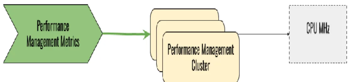
Figure 1 : Summary Representation of Earlier Study

Figure 1 shows the summary of the earlier study. This study was conducted on performance management service nodes to predict CPU consumption based defined performance management metrics. Further, the created models were evaluated using a real-world network management system, and as a result fairly accurate prediction on CPU utilization could be made.

Based on the background information there was some limitations in this early study. Firstly, the earlier study evaluated performance of CPU consumption only using multivariate regression technique. Secondly, during that stage there was limitations in collecting performance data from the software system which limited the scope of that study where only few load profiles could be tested. Thirdly, no customer data was available to compare performance levels between different environments of a created model.

3.

Background and Overview

Nokia released its initial network management tool in the early 1990s and with the evolution in network management industry it has undergone tremendous changes to date in its lifecycle. In addition, telecommunication and radio network environments became more complex in the past decades and customers are interested in accurate resource usage predictions and indicators. In some scenarios as customers only have few network element types they are interested in a minimal software setup which can fulfil their requirements without overhead nodes. Based on these facts it is essential for the business to understand the performance of each network type and management software itself.

As discussed earlier, in practice, software systems evolve with time and become complex to analyze and troubleshoot. Even though it is recommended to understand and test the performance during product development stage, in practice it is difficult as developers prioritize functionality first. In many cases product performance is only evaluated at final stages of its release lifecycle. When considering the layout of enterprise systems, they consist of complex configurations, heterogeneous communication protocols, heterogeneous and geographically distributed servers with several network interconnections, proprietary middleware, large distributed database systems, load balancers and so on which make it difficult to understand its operation on runtime. During modeling understanding its system interactions is the most difficult and important stage during the process [5].

As defined by National Institute of Standards and Technology (NIST), cloud computing enables convenient, on-demand network access to a shared pool of configurable computing resources which includes servers, network, storage, applications and services [30]. Further, these resources should be efficiently provisioned and released with minimum effort based on vendor requirements which makes every organization to step into cloud infrastructure with the growth of their businesses.

In the meantime, by leveraging cloud services, organizations can deploy their software systems to address some of their scalability and performance issues with a minimum set of changes to their systems. To achieve this application scalability, one should use scalable architecture in the first place. Microservices technology is one of the

most famous cloud native architecture which enables availability and scalability in its design by facilitating the migration of on-premise architectures to cloud environments. In addition to this, microservices can simplify business processes by including them in collection of small services which could be deployed and scaled independently, as well as different technology stacks and are easily understood [31].

3.1. Mobile Network Evolution

During the past two decades, mobile network technology has evolved drastically. This technology hype is still ongoing and expected to increase exponentially with the upcoming technologies. In recent years, big traffic volume increased in the order of several magnitudes in a short period of time due to technologies such as 5G, IoT and smart devices. During the period of 2012–2016, the yearly growth rate of the market was 78 and now, based on their marker research telecom industry expects astonishing network traffic increases after 2020 [1].

When considering these future trends, network management aspects also need to evolve with the advancements in technology. During this, accurate load models will be a handy tool in the process of designing and dimensioning software systems.

3.2. Network Management

In general, mechanisms for monitoring, control and coordination of its resources is defined by system management standards. In a telecommunications management network, its resources are viewed as independent managed objects with well-defined properties to clearly define its managed operations. This is defined by Open Systems Interconnection (OSI) - Systems management overview published by International Telecommunication Union [32]. This defines the primary requirements for understanding the key functions of network management system as a model.

For convenience, requirements and specifications related to system management is categorized into five groups by OSI Management Framework and network management model which defines these major functions of network management systems. These groups are fault management, configuration management, accounting management, performance management and security management. This is sometimes defined by the

acronym FCAPS model. The accounting management category is sometimes replaced with administration on non-billing organizations [34].

3.3. Configuration Management (CM)

This module is responsible on managing, monitoring and tracking changes on system configurations of network hardware and software elements on the system. Some possible examples are updating OS version of a network device, adding a new device to the network and modifying running configuration of a device. It is important to keep track about updated configuration changes, software versions and system changes during troubleshooting network issues, and configuration management software facilitate this. In general, configuration management facilitates [32]:

• initialize and close managed objects

• collecting, storing and change the configuration of open system

• simplifying managing configurations of the devices, associate names with managed objects

• set the parameters that control the routine operation of the open system

• assisting future expansion and network scale planning 3.4. Fault Management (FM)

To distinguish different fault scenarios, elements in the managed network consist of monitoring and diagnostic tools. Each fault in an element is represented as an event and sent to the software system. The main requirement of this module is to recognize, isolate, correct and log faults that occur in the network. In addition, FM module facilitates trend analysis on error prediction, to detect abnormalities in network operations and to configure notifications to keep the network administrator informed about problems. These notifications can be set to trigger activities that can gather more information on recognizing the nature of the fault. Fault management function facilitates [32],

• maintain and examine error logs

• accept and act upon error detection notifications

• trance and identify faults

• carry out sequences of diagnostic tests

3.5. Performance Management (PM)

To ensure acceptable level of network performance, this module should facilitate continuous monitoring of network and guarantee optimum service to mobile subscribers. The module performance addresses the throughput, network response times, packet loss rates, link utilization, percentage utilization, error rates and so on. Based on these information network managers can evaluate the current network efficiency and prepare for future network demands.

Actively monitoring current network performance is an important step to identify existing and future issues to ensure reliability during operation. In business it is important to recognize system reliability and capacity issues before they affect any services in the system. This can be done based by network health monitoring and trend analysis using system performance data. This information in management system, can be monitored in real-time, or passively by configuring to alert based on predefined thresholds when performance deviates from the expected range. Furthermore, performance thresholds can be defined to trigger alarms depending on the severity level of the events which can be handled by the FM module. Performance management function facilitates [32],

• gather statistical information

• maintain and examine logs of system state histories

• determine system performance under natural and artificial conditions

• alter system modes of operation for the purpose of conducting performance management activities

3.6. Security Management

This module guarantees the basic security requirements of confidentiality, integrity and availability of its elements considering its users, data, software and network. This includes managing network authentication, authorization, and auditing to set correct permissions to access permitted network resources based on pre-defined security policies. Security management module is responsible to ensure network environment security and gathering security-related information to be analyzed. Security management function facilitates [32],

• creation, deletion and control of security services and mechanism

• reporting of security relevant events 3.7. Accounting Management

This module enables charging capability to be established for the use of resources in open system interconnection environment, and for costs to be identified for the use of those resources. Accounting management function facilitates [32],

• inform users of costs incurred or resources consumed

• enable accounting limits to be set and tariff schedules to be associated with the use of resources

• enable costs to be combined where multiple resources are invoked to achieve a given communication objective

3.8. System Architecture

Figure 2 : Network Management System Architecture Diagram [33]

By its architecture, network management system has a modular based software system, which enables customers to customize required software features based on their

business requirements. These software modules are categorized into four main components based on the system management specifications as configuration, fault, performance and security management. Even though initial versions of a network management system were running on a dedicated hardware on physical servers, currently the system is running on the top of a virtualized environment aligning its way towards a fully automated cloud environment. This enables efficient resource allocation, scalability, reduced downtime, disaster recovery and ability for automation.

Through its southbound interfaces, communication happens between network elements and lower level systems of the managed network. This is mainly to obtain and provision data from the network. Further, the interfaces used to communication between software system and network elements are typically proprietary. Like in any other Infrastructure as a Service (IaaS) system, the hardware resources perform by means of pooled resources for the virtualized environment. The bridge between hardware and virtualized machines achieved by the virtualized layer. The northbound interfaces facilitate integrating software system with high level systems used for service management.

3.9. System Hardware

The software system can function independently from the underlying hardware resources due to its virtualized architecture. the division of hardware resources to virtual machines (VM) with a designated amount of hardware resources is handled by the platform virtualization software. Each virtual machine is allocated as per the configured amount of hardware resources to perform the intended task and these configurations can be defined as required based on the role of the individual VM.

3.10. System Performance

Performance is an indicator of how well the software meets its requirements for timeliness. System performance can be defined as a system’s capability to handle effectively the tasks that it has been assigned to do in a timely manner. Response time and throughput is used to measure the timely manner of the performance, and utilization metrics are used to measure the resource consumption. Moreover, the response time is defined as the time required to respond to an incoming request whereas throughput is the measure on how many requests can be processed in each time interval. Performance

parameters can be selected based on characteristics which influences system performance. In short, performance metrics are categorized based on above criteria’s [6].

In software systems, there can be many parameters which affect system performance. Because there can be dozens of parameters, it is important to precisely select important parameters and their effect on performance. Furthermore, based on domain knowledge and earlier studies, certain parameters can be omitted or combined to create new features. During feature extraction process, statistical methods such as Principal Component Analysis (PCA) or Canonical Correlation Analysis (CCA) can be used. Based on an initial study, selected set of important parameters are shortlisted to examine during the analysis process as this will provide more simplified and generalized performance models.

3.11. Software Metric / Parameter

Standard measure of some characteristic or properties in a software system/ process can be defined as a software metric [35]. By defining metrics, different reproducible and measurable entities are expected to be obtained which could be used to have several applications in business analysis including software performance optimization.

In any business analysis process, it is really critical to understand and select important metrics to the business process. The ‘HBR Guide to Data Analytics Basics for Managers’ written by Harvard Business Review states “You can’t pick your data, but you must pick your metrics.” which implies the importance of defining proper metrics in any analytical study. In his presentation, Haff has presented some important rules when defining metrics [36].

• what’s important to business/success criteria

• tied to business outcomes

• traceable to root cause(s)

3.12. Performance Metric

Performance metrics can be split into three main categories as time consumed on a given task, service performance rate and resource consumption of the service. In a short form, this can be defined as responsiveness, productivity (throughput) and utilization metrics [6].

When considering performance of a distributed computer system, the important operations to developer and system administrators are mainly corresponding to cluster health, resource utilization, performance and outages. Further when analyzing the system, following principles are important to consider:

• Define what you need to measure

• Selecting relevant metrics

• Quantity may not lead to quality of the process

• Understanding about what different measurements serve on different purposes

• Understanding how measurements drive behaviors

Performance parameters are measured mainly as utilization metrics corresponding to hardware performance and productivity metrics corresponding to workload. These performance parameters are later taken into account when deciding system capabilities and capacity analysis which will eventually decide on software dimensioning process. In Unix based systems, SAR (System Activity Report) system monitor command is widely used to collect and report system activity information. To record utilization metrics, SAR command is actively being used in computing as it not only has a wide range of measurements consisting of system load, CPU activity, memory, network I/O, disk I/O etc., but also it is easily integrated using sysstat package. To measure productivity metrics, software tools are used and these metrics are corresponding to performance management (PM) data (measurements and counters) and fault management (FM) data (events) discussed earlier.

3.13. Data Types in Network Management System

Even though the network traffic on mobile networks is caused as a result of its subscribers, in network management system it is different from this. The traffic on software system is based on its managed network elements such as network

performance, network failure or configuration change operations. This traffic enters the software system through its southbound interface. In this experiment PM data and FM data are mainly focused and these metrics are considered as the predictor variables during the modeling process.

Performance Management Data (PM Data)

Performance management data represents metric measurements composed by different network elements as counters. These metrics comprise of events, success rate, reset events, resource usage, signaling, etc. This measurement information can be pre-processed or post-pre-processed in the network element based on the configuration and the type of network element. Measurement can be directly uploaded to the network management system’s database as well. In addition, monitoring subscriber operations using PM data can be done by observing usage values of available services. When making management decisions based on service usage and when identifying current or future problems and opportunities, this information can be taken into consideration.

Fault Management Data (FM Data)

Fault Management data or shortly FM data mainly consist of events which can be categorized into several types for example, cancel, acknowledge, un-acknowledge and as a result FM events and alarms will be created in network management system. These alarms, when triggered represent a problem or error in a network element. In analytical perspective every FM event types are equally valued. In real life networks there could be correlations between FM and PM data as performance of the managed network can be affected by the number of fault events and the fault situation.

System Performance Data

In addition to network performance data types (PM and FM data), one can measure the data metrics related to system level performance of individual subsystems of the network management system. In practice this can be done based on individual virtual machine level considering its performance. The response variable data used in the study i.e. CPU utilization, memory consumption, disk I/O operation averages, Network I/O operation averages and response times are considered in this category.

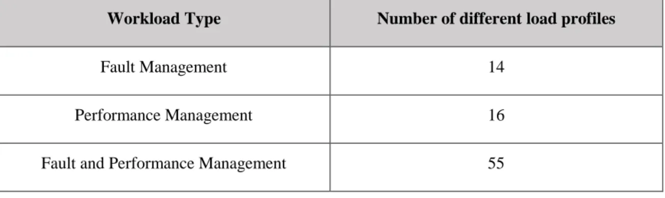
3.14. Workload Data in Network Management System

Performance data in network management system can be divided into two categories, namely simulated workload data and actual workload data. The simulated workload can be synthetic and generated in a controlled and repeated fashion. The actual workload data consist of performance data corresponding to customer environments under real life operating environments. On capacity analysis process and modeling, data sets consisting of high variance will be useful since it will help to understand system boundaries. However, since in customer environments most cases run on given boundary levels, there can be less variance in the data. Due to this reason simulated workload data can be collected and used during analysis under controlled environment conditions. As it is flexible to variate incoming data rates to the system with well-defined simulated loads, the system can be analyzed iteratively to understand its overall behavior in a detailed manner.

When simulating workloads, an instruction mix is a specification of various instructions and their relative frequency defined based on the requirement. This can be constructed for the comparison of different processors on a given hardware environment. This approach can be utilized in a distributed computer system. [6]

Exploratory Statistical Modeling and Predictive Analytics

Based on the expected functionalities and operating conditions of the data models, model building procedure leads to numerous variances in explanatory modeling and predictive analytics methods. Depending on the context, models will contrast based on explanatory power of the models vs. predictive power of the models. There are two key differences between explanatory versus predictive analysis. The first difference is the properties lie in the data used in analysis where exploratory power is being assessed by means of in-sample goodness of fit procedures. In predictive analysis prediction accuracy measures are evaluated based on out-of-sample prediction procedures.

The second difference is in the metrics used in two techniques. Even though statistical significance is an important property when assessing exploratory power, it is not so important when assessing predictive performance. In addition, Wu et al. [37] theoretically justify that sometimes removing statistically significant predictors with small coefficients could result in improved prediction accuracy. Figure 3 1 shows some differences between two techniques with respect to different states of the analysis.

4.

Overview on Machine Learning

In the next few sections, machine learning algorithms used in data modeling task in the research work and software tools used for data mining are discussed shortly.

Machine learning applications in business

In any organization, a large amount of data is produced and accumulated over time in their system. This gives businesses an opportunity and competitive advantage to extract business knowledge from underlying data. Even though it is demanding to process this data, analyzing them in a timely manner is beyond the capabilities of traditional analysis methods used by many organizations. Advancements in modern machine learning and big data techniques have enabled processing databases with large volumes in efficient fashion, leading businesses to invest on knowledge discovery applications in business.

Data mining analytic techniques are evolving with time to meet new requirements and better accuracies for different use case. This enables ability to automate decision support systems in business processes with the help of integrated analytics and optimization algorithms. It is essential to process exponentially growing data volumes in real time as IBM forecasts the growth of next decade to increase from 800,000 petabytes to 35 zettabytes [39]. This motivates businesses to invest on processing data to acquire business intelligence which could help their business with modern advancements in technology. In addition, domain knowledge contributes the business analysis process to a success as it plays an important role during the process. In his study, Weiss [40] has discussed the importance of including domain experts in data mining study to improve effectiveness of the process.

4.1. Feature Selection and Extraction

In empirical modeling and machine learning, feature (variables, predictors) subset selection is done to select a subset of most relevant features during the model creation process. This will help to improve the interpretability of the constructed model. The idea of the process is to remove any redundant or irrelevant features without suffering much information loss from the original data frame, as it could consist of many features.

Redundant features are distinct from irrelevant features as, the redundancy could be due to presence of another strongly correlated feature [41]. Feature selection techniques can help when there are many features compared to the available sample data points in the data set. Feature selection stage is important as it will:

• simplify the constructed model

• reduce training time

• address curse of dimensionality

• To make models more generalized by reducing overfitting

During feature extraction, new informative and non-redundant features are derived based on of original features. One popular example for feature extraction is ‘principal component analysis’ which is inspired by statistics. There exist a few algorithms and variations that can be used for feature selection and extraction. Further, the result feature subset can be different based on the algorithm and properties of the data. In the next section some well-known feature selection techniques are discussed.

Exhaustive Feature Selection

The brute force technique is used on subset selection to generate every possible combination of feature subsets. This process guarantees to find the best fitting subset but as a drawback the cost of the process is high. The computation cost approximately doubles by adding one additional variable as for k number of features there will be 2k- 1 possible subsets [42].

To reduce the computation cost without any information loss, there are few options available in exhaustive feature selection. Firstly, as it’s less probable that a single response variable has many statistically significant predictor variables which equally improve the models, domain experts can help to assess on limiting maximum subset size. Secondly, effectiveness of the branch-and-bound search algorithm can be improved. These two steps can be helpful to improve the efficiency of the feature selection algorithm up to large datasets [42]. The branch-and-bound algorithm will evaluate best fitting subsets up to number of feature count. The computation cost is significantly reduced in cases where only few features are dominant compared to others.

Forward Selection and Backward Elimination

In wrapper methods a feature subset is used to train a model using input features. Iteratively by inferencing the created model, the feature selection algorithm will add or remove input features form its initial feature set. Even tough, the problem can be simplified to a search problem it can be computationally expensive. These wrapper methods can be categorized as forward feature selection and backward feature elimination which will be discussed next.

• Forward Feature Selection

The algorithm starts with empty features set and iteratively adds most significant feature to the model to improve its performance. This step will be repeated until no improvements made to the model by adding of a new feature and final feature set will be selected at this stage.

• Backward Feature Elimination

The algorithm starts with all the variables in its feature set and iteratively remove least significant feature from the model to improve its performance. This step will be repeated until no improvements made to the model by removing of an existing feature and final feature set will be selected at this stage.

Efficiency of these two methods is sometimes argued in comparison to each other. Some claim that forward selection is more efficient as opposed to defenders of backward elimination who claim that weaker subsets can be found by forward feature selection as the significance of variables are not assessed compared to variables not included yet [41].

4.2. Data Mining Tasks

The main categories in data analysis tasks are descriptive, predictive and prescriptive analysis [43]. In descriptive analysis task the purpose is to provide insight to business and its stakeholders based on the past data to understand any patterns which describe the phenomena related to the data [44]. In the case of predictive data analysis, the objective is to discover any patterns that can predict the unobserved future patterns. The predictive models can be utilized by organizations to make knowledge-driven proactive decision making to the questions that were complex or time consuming in general [45]. Further, by prescriptive data analysis, steps can be utilized to optimize

current procedures and to decide next steps when decision making is executed. Several data mining techniques can be presented as follows:

• Classification – The classification algorithm will map (classifies) the input data

items into a pre-defined set of categories or classes. Some sample application would be identification of hand written digits from a large set of digit images. Once the model is developed it can be used in future inputs to recognize the digit in input image.

• Clustering – Clustering is a descriptive task where algorithm tries to identify a finite number of categories or clusters which could describe the data. This process is an unsupervised learning algorithm and output category is not known initially. In practice it is widely used in marketing to identify similarities between customers based on their purchase history and in many medical research studies.

• Prediction – Predictive models can be used to predict future trends or unknown

conditions based on its past data or as a correlation of depending factors. For example, by using an effective predictive model to predict performance, business turnover or sales can help business to prepare for unseen future challenges.

• Anomaly detection – This technique can be used to detect significant differences

compared to previously recorded data or reference levels on a given phenomenon. This technique is widely used in financial industry for fraud detection

• Summarization – This technique can be used to generalize or abstract the data

into a simplified overview and comprises on providing compact description for a of dataset. This can be as simple as determining the mean and standard deviation for a feature in a table, to more sophisticated methods involving multivariate visualization methods.

• Dependency modeling – This technique can be used to find models that has

defined based on structural level or quantitative level of the models it specifies. The features that are locally dependent on each other and variable strengths of the dependencies will be evaluated in these two cases [44].

4.3. Machine Learning Algorithms

In this section, brief introduction on data mining and machine learning techniques which were evaluated during the modelling process are discussed. As the initial base predictors for modeling task, six machine learning algorithms were used. These algorithms are multiple linear regression, MARS, k-nearest neighbor, random forest, support vector regression and feedforward neural networks. To train the data models, supervised learning techniques were used. In supervised learning, every entry in the data set consists of precise output values which are used to train the models accordingly [46]. Introduction about selected machine learning techniques is presented below.

Multiple Linear Regression

In practice, descriptive modeling as well as predictive modeling is done using Multiple linear regression [48]. The model is constructed against response variable from a sample of data points, corresponding to its input variables. Most simple technique used in linear regression is the ordinary least squares method, which aims to minimize sum of squared error on model creating. Descriptive modeling uses available set of data to model existing features from the data. During predictive modeling, response variable values for new cases are predicted based on model constructed by existing predictor variables. The sample equation of multiple linear regression represents its response variable as a linear combination of its predictor variables. Below is a sample equation with p predictor variables:

Y = β0 + β1X1 + β2X2 + ……. + βpXp + ε (1)

Equation 1 : Equation of Multiple Linear Regression

In the above equation, response variable is denoted by Y and the predictor variables are denoted by X’s. Further, β0 denotes intercept and remaining β values

represent the coefficients of each predictor variable. The error of the model is represented by ε. The process of predicting more than one response variables at once is

known as multivariate linear regression analysis. Multiple linear regression and multivariate linear regression modeling are two distinct techniques and should be used appropriately [49].

In multiple linear regression, to make reliable predictions with two or more predictor variables, the input data set should satisfy additional qualities compared to modeling using simple linear regression. The efficiency of the method depends on the ability of presenting the response variable as a linear combination of the predictor variables. The statistical significance of the model test can be disturbed by lack of linearity which causes model fit, errors and residuals. Further, to prevent multicollinearity, the predictor variables should not be correlated among each other and this can be detected through the variance inflation factor [50]. In addition, there can be situations where outlier data points get recorded due to measurement errors or unmeasured metrics [51].

Multivariate Adaptive Regression Splines

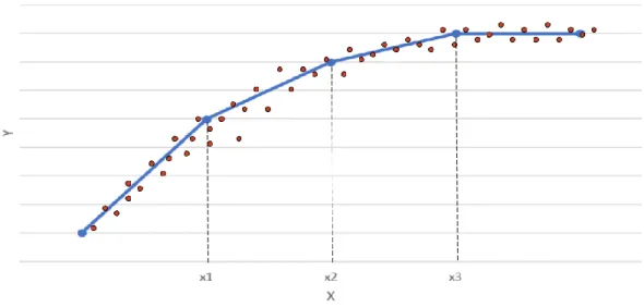
Multivariate adaptive regression splines (MARS) technique introduced by Jerome H. Friedman is a parametric regression technique. It’s capable of modeling non-linearities and relations among features represented by the input data. MARS method builds models of the form as below,

f̂(x) = ∑𝒏_𝒊=𝟏𝒄𝒊 𝑩𝒊(𝒙) (2)

Equation 2 : Sample Equation of MARS Method

The model is represented as a weighted sum of basis functions Bi(x) where ci is a

constant coefficient multiplied by its basis function. Each basis function can take one of the following three forms:

1. a constant

2. a hinge function. A hinge function has the form max (0, x-const) or max (0, const-x)

Figure 4 : Sample Model Representation using MARS Model

The term "MARS" is trademarked and in order to avoid trademark infringements, many open source implementations of MARS are called "Earth".

K-Nearest Neighbors (K-NN)

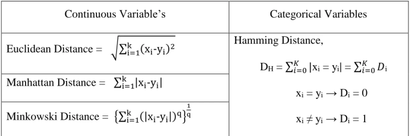
K-Nearest Neighbor algorithm is an instance based learning (IBL) technique, which is considered as one of the simplest methods. From the available data set all the known cases are stored by the algorithm to solve new cases. To determine the result for an unknown case, the algorithm will compare it with the similar instances in the training data. Further, this algorithm will assume that data points with similar attributes exist in close proximity compared to others and these nearby data points are called neighbors [46]. When predicting the class label for a new instance, the algorithm searches for K nearest training samples that are close to the new instance, and most frequent class value is assigned. Further, Euclidian distance or Cosine similarity can be used as similarity measure [52]. In practice different variations of distance functions being used are based on domain knowledge and properties of the data. Evaluating continuous variables should be done using Euclidean, Manhattan, Minkowski distance measurements and evaluation of categorical variables should be done using Hamming distance, which measures the number of instances of corresponding symbol or category. The K value used in the algorithm is a small positive, usually an odd number. The simplest way to select a suitable K value is to iteratively run the algorithm on different K values and select the one with the highest performance [48].

Determining an optimum K value is based on few criteria. Firstly, a suitable value for K can be selected by inspecting the data itself. In many practical scenarios cross-validation of performance for each K value will be evaluated iteratively based on independent input data set and suitable K value will be selected. In general, a large K value will be more precise as it can reduce the overall noise depending of the distribution of data. However, distinction between boundaries within the feature space also needs to be considered [53]. A rule of thumb to select a maximum for K is to use √n if nothing about a suitable value is known in advance where ‘n’ is equal to data items.

Distance Techniques for Continuous Variable’s

Continuous Variable’s Categorical Variables Euclidean Distance = √∑ki=1(xi-yi)2

Hamming Distance,

DH = ∑𝐾_𝑖=0|xi = yi| = ∑𝐾_𝑖=0𝐷i

xi = yi → Di = 0

xi ≠ yi → Di = 1

Manhattan Distance = ∑ki=1|xi-yi| Minkowski Distance = {∑ki=1(|xi-yi|)q}

1 q

xi, yi = Coordinates or values of data points k = Number of cases

Table 1: Distance Techniques

Random Forest

A random forest model is an ensemble learning technique that can be used on both classification and regression tasks. During learning stage, the algorithm constructs several decision trees and produces the output class which is the most occurring class for classification and mean prediction for regression tasks. A Random Forest with few trees is quite prone to overfit to noise and once more trees are added, the tendency to overfit generally decreases [54]. Random forest models make use of random selection of features in splitting the decision trees, hence the classifier built from this model is made up of a set of tree-structured classifiers.

When constructing a model using the algorithm, random k data points from the training set are taken and a decision tree is built associated with these k data points. Next, by selecting the number of trees (ntrees) desired to be built and the earlier steps are repeated. When classifying a new data point, a prediction is made on category to which the data point belongs using earlier ‘ntrees’ and will be assigned to the winning class. This process will start by one tree and then proceed to build more trees based on the subsets of data. The random forest has a major advantage that it can be used to judge variable importance by ranking the performance of each variable. The model achieves this by estimating the predictive value of variables and then scrambling the variables to examine how much the performance of the model drops.

Support Vector Machine

Support vector machine is a supervised learning method. There are two flavors of this technique which can be used to analyze both classification and regression problems. Firstly, support vector machine (SVM) can be used during classification problems. Secondly, support vector regression (SVR) can be used during regression problems with minor differences in the concept containing of all main features which are based on maximum margin algorithm. The algorithm will construct a nonlinear function based on linear mapping into a high dimensional kernel inspired from the input feature space. The parameters will control the capacity of the system. In addition, these parameters do not depend on the dimensionality of the input feature space.

During the training process of SVR classifier, algorithm will iteratively improve the support vector function. The optimization can be controlled using a tolerance parameter (↋) to set an approximation to the SVR. If the gradient of the optimized function is less or equal to the tolerance parameter value, the training is terminated. If the tolerance value is large the training algorithm can terminate before support vector function is sufficiently optimized, and for lower tolerance value, algorithm could try to attain high optimization levels which will be computationally expensive and time consuming.

Figure 5 : One Dimensional Linear Regression with Epsilon Intensive Band [55]

In models created by support vector, models only depend on a subset of the training data. During classification task, the cost function on building the model ignores training data points lying beyond the margin. Analogously, during regression analysis, the cost function on building the model ignores training data points adjacent to the model prediction.

Figure 6 : Non-linear SVR Representation [55]

The estimation accuracy and performance of support vector depends on its input setting of parameters such as C, ↋ and the kernel parameters. As support vector model is

a complex algorithm, the selection of optimal parameters is further complicated. In software implementations of support vector regression, these meta-parameters are given as user defined input parameters. In addition, selection of the kernel type and kernel function parameters are typically derived to reflect the distribution of the input training data and based on application domain experts [55]. Two non-linear kernel functions used during the study are presented below.

Polynomial Kernel Function = 𝒌(𝒙_𝒊, 𝒙_𝒋) = (𝒙_𝒊. 𝒙_𝒋)𝒅 (3) Gaussian Radial Basis Function = 𝑘(𝑥𝑖, 𝑥𝑗) = 𝑒𝑥𝑝 (

||𝑥𝑖− 𝑥𝑗||𝑑

2𝜎 ) (4) x_i, x_j = Coordinates or values of data points

Equation 3 : Polynomial Kernel and Gaussian Radial Basis Function

Artificial Neural Networks

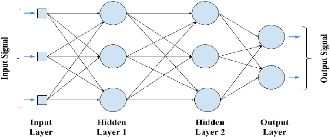
Artificial Neural Network (ANN) technique and its configurations are inspired by functioning concepts of human brain, as human brain can be observed as a connecting mesh of neurons and synapses. Neurons are considered as computational units where synapses operate as the signal transferring unit. In general, every neuron is connected to several other neurons by these synapses. Even though, neurons and synaptic connections inside human brain are connected in an unorganized fashion, in ANN neurons and synapses are structured in organized way to design computationally manageable system. Sample configuration diagram of an ANN is shown in Figure 7.

As the presented diagram neurons are organized in layers. The structure of neural network consists of one input layer followed by one or more hidden layers and finally an output layer. The simplest network would consist of two layers and once the network become more complex number of hidden layers will be increased to two or three (more are not necessary). The network in Figure 7 has four layers which consist of two hidden layers.

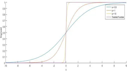
When connecting input nodes or neurons of a neural network, they typical way is to connect all nodes of the previous layer to the next layer where each connection is assigned a weight. These types of networks are known as fully connected network and Figure 7 demonstrate such network. A neuron or node computes the sum of the outputs from neurons in the previous layer multiplied by the weights assigned by the connections, and then passes it to an activation function. Activation functions enable ANNs to learn non-linear functions. There are different activation functions, e.g. sigmoid function. The effect of a sigmoid function is demonstrated in Figure 8 where activation function outputs value between 0 and 1.

Figure 8 : The Effect of Slope Parameter in Sigmoid Function

A neural network supports both supervised learning (for networks such as one in Figure 7) and unsupervised learning techniques. Self-Organizing Maps (SOM) is the most well-known application in unsupervised neural networks. The available neural network types can be mainly categorized into feedforward and feedback networks.

Feedforward neural network is a non-recurrent network which consists of input, output and hidden layers where input signals only travel in one direction. First, inputs are assigned to input nodes and then they are passed into first processing layer of nodes. When designing a network, the number of input and output neurons is equal to the number of input and output variables in the network. The computations inside a neuron is done based on the weighted sum of its input data and this output value become the input values which fed into the preceding layer. This procedure will be followed iteratively through all layers and finally determines the output values. In practice, threshold transfer functions are used to quantify the values of output layer. In data mining problems, feed-forward networks are generally used. In addition, feed-forward networks (FFN) also include Perceptron and Radial Basis Function networks.

Feedback networks consist of loop like paths which can transmit the signals in both directions between layers allowing all possible connections among neurons. Due to these characteristics the network becomes a non-linear dynamic system with continuous changes until the network reaches a state of equilibrium. These feedback networks are generally used in optimization problems and associative memories [56].

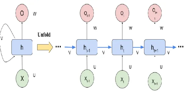
Recurrent Neural Network (RNN)

Recurrent neural networks can process sequences of inputs as the networks use their internal state (memory) by feeding back the output signal of the neurons to the neurons in the same layer. This enables the network to exhibit dynamic temporal behaviors on a given time sequence. RNN’s are generally applicable in unsegmented, connected handwriting recognition or speech recognition problems. There exist many possibilities of connecting feedback between neurons and some common ways are:

• Self-feedback: Along with the next input data sample, the output signal is fed back into the same neuron.

• No self-feedback: Along with the next input data sample, the output signal is fed back to all other neurons of the same layer except the neuron itself. This case is illustrated in Figure 9.

• Full feedback: Along with the next input data sample, the output signal is fed back to all other neurons of the same layer.

5.

Methodology

In this chapter, the methodology used during the study is presented. The main objective of the study was to create descriptive performance models of a software system to understand its behavior based on business usage and requirements. In theory, not only ‘Analytical Performance Modelling’ concepts can be used to model system operation, but also to performance testing as a faster and economical option. Once we have the required understanding about the hardware utilization based on our models this can further be used on evaluating design options and system sizing [57].

As discussed earlier, currently system dimensioning and performance is being predicted mainly based on an expert’s knowledge and it would require manual work and methods can be biased and many practicalities were reported which encouraged Nokia to research more data intensive approaches. Even though the current dimensioning tool supports complex network design, it not only requires continuous maintenance but also testing to adopt changes which makes the process tedious. Further, over or under estimations in system capacity can create business impact not only on revenue but also on customer loyalty. As the ultimate result of the study, in addition to system level behavioral knowledge, stakeholders can estimate system scalability based on workloads. Based on the market research and domain knowledge by the experts, Nokia expects that in the future customer environments can be substantially different from one another. With the advancements in cloud computing systems can evolve to fine granted tailor-made customer environments (e.g. microservices) which are more economical for their business needs. Developing accurate performance models can contribute on precise dimensioning needs where customers can efficiently use available system resources in their business which customers will definitely appreciate. It is expected to iteratively improve system understanding by continuous studies that can ultimately result new dimensioning technique which can overcome limitations in current dimensioning solutions and perform well with future business needs. This study is only one iteration for that process and the study is mainly focused on evaluating the goodness of different data mining and machine learning techniques on performance modelling of Nokia’s network management system. Further, during modelling the system performance