Circular(2)-linear regression analysis with iteration order manipulation

(1)

Circular(2)-linear regression analysis with iteration order

manipulation

Muhamad Irpan Nurhab a,1,*_{, Badaruddin Nurhab}b,2_{, Tuti Purwaningsih}c,3_{, Ming Foey Teng} d,4

a _{Department of Economics, STIE MURA, Indonesia} b_{Department of Economics, IAIN Bengkulu, Indonesia}

c_{Department of Statistics, Universitas Islam Indonesia, Indonesia} d_{American University of Middle East, Kuwait}

1_{[email protected]*;}2 _{[email protected];}3 _{[email protected];} 4 _{[email protected]} * corresponding author

I. Introduction

A model of distribution and statistical techniques for analyzing random variables in the form of cycles in nature is Circular statistics. Circular statistics are used on data whose measurement results are directions and are usually expressed in angle size. This technique has evolved in several fields of science where exploration, modeling and hypothesis testing of the direction and angle data play an important role.

The presentation of data in two-dimensional directions is not a single angle or unit vector because the angular value depends on the choice of starting point specified as the angle 00 and the direction of rotation. A mathematician considers the 600 direction measured from the west as the starting angle and the direction of rotation counterclockwise, but the direction of the same position is considered to have a direction 300 by a geologist measured from the north as the starting angle and rotates clockwise [1].

Circular data can be expressed in several ways. The usual way is related to two circular measuring instruments, ie compass and clock. The observed form is measured using a compass such as the direction of the wind and the direction of bird movement, including the data measured using a protractor. Forms of observation measured by hours may be time, eg arrival time (24 hours) of patient in emergency room at a hospital and number of incidents in one year or in monthly time [2]. Brunsdon and Corcoran [3] use circular statistics to see the timing patterns of criminal acts in both daily and weekly times.

Some distributions in circular statistics are uniform distribution, wrapped distribution, distribution of cardioids and distribution of von Mises. One of the most widely used distributions is the distribution of von Mises. Like the normal distribution of lines, the distribution of von Mises has an important role in descriptive statistics and the statistics of circular inferences.

ARTICLE INFO A B S T R A C T Article history:

Received July 18, 2017 Revised August 21, 2017 Accepted August 21, 2017

Data in the form of time cycle or point position to the angle of possibility is no longer suitable to be analyzed using classical linear statistic method because the direction and the angle influence the position between one data with other data. This paper aims to examine the comparison of Linear Regression Analysis with Circular Regression Analysis. The writing method used is literature review using simulation data. Data simulation and analysis is done with the help of R program. The results showed that circular data is better analyzed by Circular Regression Analysis rather than Classical Linear Regression Analysis. The use of classical linear statistic method is not recommended due to the direction and the angle influence the position between one data with other data.

data circular

circular(2)–linear regression simulation

(2)

The study of this research aims to examine the comparison between Linear Regression Analysis and Circular Regression Analysis. More specific this model will be bring to Circular Regression(2)-Linear Order 2. This paper will give new information about the possibilities to have a better prediction when manipulate the order of iteration. It works as the new approach for improving value of R2_.

II. Literature Review

A. Data and Circular statistics

Circular data is the data of measuring result that the values always repeat periodically. The value will be found again after meeting a full period. The definition of circular variable itself is data in the first and the last scale which meets each other [4]. The circular data is divided into two types, direction-circular data and time-direction-circular data [4].

Circular statistics is a distribution model and statistical technique to analyze random variable of the cycle in the nature. Circular statistics is used on data which has direction-measurement output and is usually expressed in angular size. This technique has developed in some branches of science in which exploration, modeling, and hypothesis trial from directional data and angle have crucial role.

Von Mises distribution is the normal spread of circular with dispersion using (1).

) cos( 0 0( ) 2 1 ) , ; (   











_  e I g   

The method used to evaluate Von Mises dispersion is QQ-plot by finding Zi using (2) then Zi is arranged based on the minimum grade to the maximum grade until Z1 ≤ ... ≤ Zn and after that make

plot using (3).













_i i

Z

2

1

sin



i



1

,

2

,...,

n

  

















































n n

Z

q

Z

q

,

2

1

sin

,...,

,

2

1

sin

₁ ₁   

If the data follows Von Mises distribution, plot will follow the straight line (0,0) in declivity 450 [5]. Data could be easily analyzed if it is illustrated on a graph. According to [5], the representation of circular data on a graph is very important in the analysis of circular data.

To analyze circular data, two trigonometry functions used as the foundation are sinus and cousins. Both two functions are utilized to position the data. Those functions are used to harmonize 2 coordinate systems. Jammalamadaka and Sengupta [1] state the directional position could be determined by polar coordinate or Cartesiancoordinate. In Cartesian coordinate, P point is stated as value (X,Y) or value (r,θ) on polar coordinate by which r is the distance of P point from the center point O. Polar coordinate can be converted to Cartesian coordinate by using trigonometry (4). The relation between cartesian coordinate and polar coordinate shown in Fig 3.



,

sin

cos

y

r

x



_ _ _

In circular analysis, the concerned thing is direction, not vector quantity. Consequently these vectors are changed to unit vector which is a vector that has length unit with r = 1. Every direction has a connection with P point in the circumference of a circle. Conversely, this point in the circle circumference could be named as an angle. If P point is situated in the circle circumference, the change of polar coordinate and Cartesian coordinate using (5).

α)

α,y

(x

,αα

(3)

The average direction of the circular sample data is obtained by calculating the vector resultant of unit vectors from each sample. The direction of vector resultant shows the average way of data sample, and the average length of resultant from each sample describes the concentration of data against the average direction. For example, there are samples

𝛼

1

, 𝛼

2

, … , 𝛼

𝑛 with n circular observation stated in angle. Known the transformation from polar coordinate to Cartesian coordinate for each observation using (6). n i y x i i i) ( cos , sin ), 1,2,..., , 1 (



 







 _ _ _

The result is the resultant vector from vector unit by summing up for each component using (7).

𝑅 = (



 n i i 1 cos



,



 n i i 1 sin



) = (𝑪, 𝑺) (7)

with R is calculated using (8),

n R S C R R  2  2,0    

R stands for the length of resultant vector R that is calculated using (9),

1

R

0

,

n

R





  

where

R

stands for the average length of resultant vector and also shows the concentration measure from data against average direction. The direction of vector resultant R is the direction of circular mean that is symbolized by  and defined using (10),

cos 𝛼

₀

=

𝐶

𝑅

, sin 𝛼

0

=

𝑆

𝑅   

For more explicit it is given inverse “quadrant-specific” from tangent using (11),













            undefined C S C S C S C S





2 / arctan / arctan 2 / / arctan arctan* 0

if

0

,

0

,

0

,

0

,

0

.















S

C

S

C

S

C

S

C

(11)

If all dot angles show the same direction, so that data is concentrated and R is close with n. On the other hand, if data spreads in all circle, therefore it is not concentrated and R verges on 0 [1]. On [4] defined the mode of circular sample is V = 1-

R

. As smaller the value of circular mode, as concentrated the data into a certain point. The value of V is on interval [0,1].

B. Simple Linear Regression (SLR)

Simple linear regression different with multiple linear regression, the difference is in number of explanatory variable. Data used in this model are scalar, mentioned as y as the dependent variable and X as explanatory variable. SLR develop a model between Y and X [6].

SLR model have many practical uses. There are two broad categories which commonly used by data analyst:

(4)

a. For prediction purposes, the X variables as input variables to the SLR. Y as the response variables usually need to be predict at the next period if time series data, and next object as cross-section data. The model will be good if the R2_{value bigger than other}

b. To know the strength of relationship/ influence from X to Y variables. The bigger SLR coefficient is representing the bigger influence of X too.

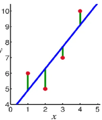
Fig. 1 illustrates the relationship between Y data and X data, it is show us that X and Y have positive correlation in the picture. At the picture there are three items we have to know, the first is the observations as data shown as red, it consist of X and Y data. Second is regression line, this line estimate which position is the best for represent the relationship between X and Y, the third is error. The error symbolized as the distance between red and regression line [7].

Fig. 1.Illustration of how error in linear regression Linear Regression can be defined as in (12) [6].



Y

i





0





1

X

i





i  

The attribute for equation (12) consist of

Y

i_,

X

i_,

Y

i_,



0_,



1_and



i_.

Y

i_{is dependent variable for}

object i,

X

i_{Independent variable (predictor) variable for object i,}



0





1

X

i_{represent the linear}

relation between Yi and Xi ,



0_{and is a mean of Y when X=0 (Y-intercept),}



1_{for the slope in mean} of Y when X increases by 1 measurement and



i_{are random error terms.}

C. Circular Regression

The regression formula for circular data is divided into three options [8], they are :

1. Circular regression-linear: the regression analysis with independent variable is circular variable and dependent variable is linear variable.

2. Linear regression-circular: the regression analysis with independent variable is linear variable and dependent variable is circular variable

3. Circular regression-circular: the regression analysis with both independent and dependent variable are circular variable.

Circular regression model(2)-Linear between linear variable Y and 2 independent variables circular α can be written using (13) [9], [10].

) cos( ) cos( ) (X  A0 A1



1



01 A2



2 



02 E _ _ _{}

for example, B_k1  A_kcos



0_kand Bk2  Akcos



0k , it can be written as 2 22 2 21 1 12 1 11

0 cos sin cos sin

)

(X A B



B



B



B



E      _ _{}

(5)

2 22 2 21 1 12 1 11

0 B cos



B sin



B cos



B sin



A

Y      _ _{}

The application for circular model are many, one of the proof is studied by Linder and Williander [11].the study show about examination of causes for reluctance. They assume on a hypothesis-testing framework of business model innovation, and show the significant roles of circular business models which imply significant challenges to proactive uncertainty reduction for the entrepreneur. Moreover, the study show that many product–service system variants that facilitate return flow control in circular business models further aggravate the potential negative effects of failed uncertainty reduction because of increased capital commitments. The other study is about circular model applied in nonparametric data, studied by Di Marzio et al. [12]. Guerrero and Solar [13] applied circular data with Gaussian process. The special research did by Kim and Sengupta [10] about circular model with inversed approach and the another research came from Peiris and Kim [14] which restricting inference of Circular - Linear and Linear - Circular Regression Model.

D. Regression Coefficient Assesment

The regression coefficient A₀,B₁₁,B₁₂,B₂₁,B₂₂ can be expected by using The Smallest Quadrate Method. This method chooses its parameter value so the value of Error Sum of Squares (SSE) is minimum. The solution of this equation is the smallest quadrate assessment, such as

2 1 12 11 0

,

ˆ

,

ˆ

,

ˆ

,

ˆ

p p

B

A



[8], [15]–[17].

If The regression model of Circular(2)-Linear can be written in matrix form as (16).









Z

Y

_ _ _{} with                                           m m n b b b b b b a Y Y Y Y 2 22 21 1 12 11 0 2 1 ;   

















n





2 1 (17) 𝒁 = [ 1 1 ⋮ 1 𝑐𝑜𝑠𝛼₁₁ 𝑐𝑜𝑠𝛼₂₁ ⋮ 𝑐𝑜𝑠𝛼_𝑛1 𝑠𝑖𝑛𝛼11 𝑠𝑖𝑛𝛼₂₁ ⋮ 𝑠𝑖𝑛𝛼𝑛1 ⋯ ⋯ ⋮ ⋯ 𝑐𝑜𝑠 𝑚𝛼₁₁ 𝑐𝑜𝑠 𝑚𝛼₂₁ ⋮ 𝑐𝑜𝑠 𝑚𝛼_𝑛1 𝑠𝑖𝑛 𝑚𝛼11 𝑠𝑖𝑛 𝑚𝛼₂₁ ⋮ 𝑠𝑖𝑛 𝑚𝛼𝑛1 𝑐𝑜𝑠 𝛼₁₂ 𝑐𝑜𝑠 𝛼₂₂ ⋮ 𝑐𝑜𝑠 𝛼_𝑛2 𝑠𝑖𝑛 𝛼12 𝑠𝑖𝑛 𝛼₂₂ ⋮ 𝑠𝑖𝑛 𝛼𝑛2 ⋯ ⋯ ⋮ ⋯ 𝑐𝑜𝑠 𝑚𝛼₁₂ 𝑐𝑜𝑠 𝑚𝛼₂₂ ⋮ 𝑐𝑜𝑠 𝑚𝛼_𝑛2 𝑠𝑖𝑛 𝑚𝛼12 𝑠𝑖𝑛 𝑚𝛼₂₂ ⋮ 𝑠𝑖𝑛 𝑚𝛼𝑛2 ] (18)

where Y is the observation vector in size (nx1), Z is matrix in size (nx(1+4m)), β is regression coefficient vector in size ((1+4m)x1), and ε = error random vector in size (nx1).

Then, it needs to search the smallest quadrate assessment vector



ˆ that can minimize the function of error quadrate L using (19).









      

    X Z X Z X X  Z X  Z Z

L _i2 ' ' ' 2 ' ' ' ' _ _{}

(6)



Z'Z



Z'Y

ˆ _ 1

 _ _ _{}

The Error sum of squares (SSE) is calculated using (21) by substituting (19) to (20)

Y Y

Y

SSE ' ˆ'Z'   

E. The reduction of Error Sum of Squares (SSE)

The important thing to define the order in polynomial regression is by reducing SSE when m is increased. The decision is taken on the degree of trigonometry polynomial (m+1) by adding columns. To determine whether or not we take degree (m+1), firstly we should calculate the reduction of SSE using (21). If reduction is obviously great in number, we decide to put degree (m+1) in [8].

III. Methods

The data used in this research are simulation data and secondary data. Independent variable γ and δ simulation data is obtained by using rvm (60,0,1) in software R.3.0.1 [1].

The procedures needed to reach the purpose of this research are :

First step: creating a descriptive analysis about circular statistics for each variable γ and δ. Graphical representation of circular data for each variable γ and δ by using transmit diagram and rose diagram

 Compatibility graph of Von Mises distribution

 The average of circular and linear direction for each γ variable and δ variable  The vector length of circular average on each γ variable and δ variable using



The data mode on circular statistics and linear statistics for each γ variable and δ variable Second step: multiple linear regression analysis and circular regression(2)-linear for γ variable and δ variable as independent variable against Y linear variable as dependent variable.

The regression equation of circular(2)– linear for order m=1 using (22)

2 22 2 21 1 12 1 11

0 B cos



B sin



B cos



B sin



A

Y      _ _{}

Third step : determination of order m from circular regression(2)-polynomial linear using (23).

2 2 2 1 2 22 2 21 1 12 1 11 0 sin cos 2 sin 2 cos sin cos



m B m B B B B B A Y m m            

IV. Result and Discussion

A. Descriptive statistics simulation data γ circular variable and δ circular variable

It was shown on the average way of γ in table 1 with circular statistics about 350,730_{. While for} the average way of γ with linear statistics was around 203,470_{. On Table 1 it can also be seen the} resultant length was about 30,7 and the average length of resultant was 0,51 that indicated a big concentration value of data to the average direction of γ circular variable. The mode value on statistics circular data was 0,49 which showed the small data dispersion. However, the mode mark on linear statistics was about 17738,73 which proved the big data dispersion.

The average direction of δ variable with circular statistics was 12,970_{. In the meantime by using} linear statistics, the average way of δ was 174,070_{. It was also drawn from δ variable that the resultant} length was 28,75 and the average length of resultant was 0,48. It demonstrated the small concentration of data to the average direction on statistical circular δ variable. The mode value on circular statistics was 0,52 that indicated its small data distribution. On the other hand, the mode value on linear statistics was 17006,5 that showed the great data dispersion.

(7)

Table 1. descriptive statisctis of simulation data from γ circular variable and δ circular variable

Variable γ variable δ variable

Number of observation 60 60

Circular average way 350,730 _12,970

Linear average way 203,470 _174,070

The length of resultant 30,7 28,75

The average length of resultant 0,51 0,48

Circular mode 0,49 0,52

Linear mode 17738,73 17006,5

B. The Compatibility graph of Von Mises distribution simulation data on circular variable (γ) and circular variable (δ)

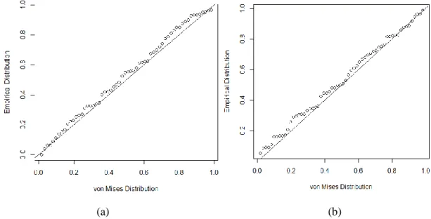
The compatibility result of Von Mises distribution that was done with Von Mises Q-Q plot on α variable and δ variable can be seen in Fig. 2, as in Q-Q plot, data for γ variable and δ variable demonstrated the data dispersion was following the straight line (0,0) in declivity 45 o, consequently it can be said that data of γ variable and δ variable was coming after the normal circular distribution or von Mises.

(a) (b)

Fig. 2. Compatibility graph of Von Mises distribution simulation data (a) Q plot graph in γ variable (b) Q-Q plot graph in δ variable

C. Representative Graph simulation data circular variable (γ) and circular variable (δ)

The transmit and rose diagram in Fig. 3 and 4 illustrated that the red-straight line was the average direction of circular statistics from γ variable which was 350,730 _meaningγ variable with circular statistics had inclination toward the north, and the black-dash line was the average way of linear statistics from γ variable which was 203,470 _{that meant γ variable with linear statistics had southward} tendency.

(8)

It proves the counting difference of the average direction on data between circular statistics at data distribution and linear statistics keeping away from data distribution.

Fig. 4. The transmit diagram δ variable

Fig 4 on transmit diagram and rose diagram were seen the red-straight line was the average direction of circular statistics from δ variable about 12,970 which meant δ variable with circular statistics had northward inclination and the black-dash line was the average way of linear statistics from δ variable about 174,070 meaning δ variable by using linear statistics had southward inclination. It indicates the calculating difference about the average direction between circular statistics on the data distribution and linear statistics sheering away from the data distribution.

D. Multiple linear regression and Circular regression(2)-Linear at simulation data to analyze the influence of γ circular variable and δ circular variable against Y variable

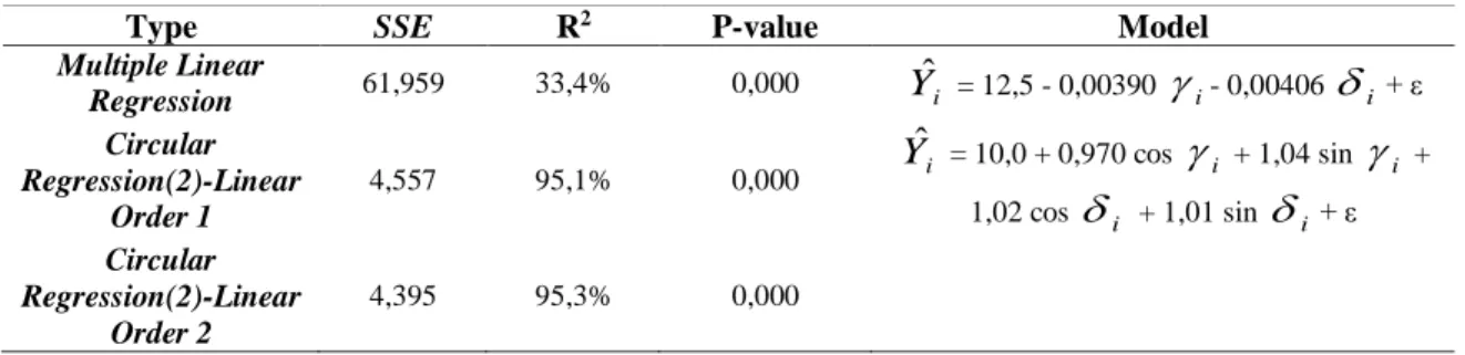
In Table 2, the value of determination coefficient on multiple linear regression was around 33,4% which it meant around 33,4% the variety of Y variable can be explained by γ and δ variable in a linear correlation, and the rest was influenced by other factors. However, the grade of determination coefficient on circular regression(2)-linear in Table 2 was about 95,1% for order 1 and 95,3% for order 2 meaning about more than 95,1% diversity of Y variable can be elucidated by γ and δ circular variable, and the rest was by other factors. From the result, we can see that circular regression(2)-linear had much better output than multiple regression(2)-linear regression to know the influence of γ and δ circular variable against Y linear variable.

Table 2. Multiple Linear Regression and Circular Regression(2)-linear on simulation data to see the influence of γ and β circular variable to Y linear variable.

Type SSE R2 P-value Model

Multiple Linear Regression 61,959 33,4% 0,000 Yˆi = 12,5 - 0,00390



i- 0,00406



i+ ε Circular Regression(2)-Linear Order 1 4,557 95,1% 0,000 Yi ˆ _{= 10,0 + 0,970 cos} i



+ 1,04 sin



_i + 1,02 cos



_i + 1,01 sin



_i+ ε Circular Regression(2)-Linear Order 2 4,395 95,3% 0,000

P-value on multiple linear regression was 0,000, so with the error possibility α = 0,1 that P-value (0,000) < α (0,1). It can be described that the model of multiple linear regression can be used significantly to see the influence of γ and δ variable to the average of Y variable with credence degree 90%. In circular regression(2)-linear with error degree α = 0,1, the P-value (0,000) < α (0,1). It means the model of circular regression(2)-linear order 1 and 2 was significantly used to know the influence of γ and δ circular variable to the average of Y linear variable with degree of credence 90%.

One of the ways to determine the best model is by using reduction method of SSE. If the value of SSE order 1 – SSE order 2 = 4,557-4,395 =0,162, it indicates that the decrease of SSE is very small so the model of circular regression(2)-linear order 1 is better than order 2. Therefore, the best model used to see the influence of γ and δ circular variable toward Y variable on simulation data was Yˆ = _i 10,0 + 0,970 cos



_i + 1,04 sin



_i + 1,02 cos



_i + 1,01 sin



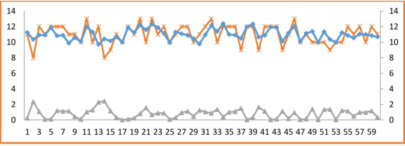
_i+ ε.

(9)

Fig. 5 illustrates the graph of Y prediction at multiple linear regression is less close on the real value of Y so creates a high error. Fig 5 shows the graph of Y prediction on circular regression(2)-linear is very close with the real Y grade. In conclusion, the circular regression(2)-regression(2)-linear possess better result than multiple linear regression on simulation data.

Y simulation data Error Y prediction simulation data

Fig. 5. The comparative graph of Y prediction simulation data, Y simulation data, and error at multiple linear regression

V. Conclusion

Diagnosis data before doing the regression analysis is an early stage should be done to determine the appropriate type of regression. The type of data that is dimensionless direction (the direction of the wind, the direction of navigation, the direction of the clouds) and time (day, month, year, time) is a circular kind of data. Data were analyzed using a circular multiple linear regression produces less regression model, when compared with the regression model generated by the circular regression (2) -linear.

Acknowledgements

We thank for all parties who support this research. With the collaboration of all parties, this research could reach its purpose.

References

[1] S. R. Jammalamadaka and A. Sengupta, Topics in circular statistics. River Edge, N.J: World Scientific, 2001.

[2] P. E. Jupp and K. V Mardia, “A general correlation coefficient for directional data and related regression problems,” Biometrika, vol. 67, no. 1, pp. 163–173, 1980.

[3] C. Brunsdon and J. Corcoran, “Using circular statistics to analyse time patterns in crime incidence,”

Comput. Environ. Urban Syst., vol. 30, no. 3, pp. 300–319, 2006.

[4] M. I. Nurhab, A. Kurnia, and I. M. Sumertajaya, “Circular Circular–Linear Regression Analysis of Order m in Circular Variable α and β against Linear Variable (Y).”

[5] N. I. Fisher, Statistical Analysis of Circular Data, 3rd ed. New York: Cambridge University Press, 1995. [6] D. A. Freedman, Statistical models: theory and practice. cambridge university press, 2009.

[7] M. Krzywinski and N. Altman, “Points of Significance: Multiple linear regression,” Nat. Methods, vol. 12, no. 12, pp. 1103–1104, 2015.

[8] Jammalamadaka, S. Rao and Y. R. Sarma, Statistical Theory and Data Analysis II: Proceedings of the Second Pacific Area Statistical Conference, 2nd ed. North Holland: Elsevier Science Ltd, 1988.

[9] A. H. Abuzaid, I. B. Mohamed, and A. G. Hussin, “Procedures for outlier detection in circular time series models,” Environ. Ecol. Stat., vol. 21, no. 4, pp. 793–809, Dec. 2014.

[10] S. Kim and A. SenGupta, “Inverse Circular--Linear/Linear--Circular Regression,” Commun. Stat. Methods, vol. 44, no. 22, pp. 4772–4782, 2015.

0 2 4 6 8 10 12 14 0 2 4 6 8 10 12 14 1 3 5 7 9 11 13 15 17 19 21 23 25 27 29 31 33 35 37 39 41 43 45 47 49 51 53 55 57 59

(10)

[11] M. Linder and M. Williander, “Circular business model innovation: inherent uncertainties,” Bus. Strateg. Environ., vol. 26, no. 2, pp. 182–196, 2017.

[12] M. Di Marzio, A. Panzera, and C. C. Taylor, “Nonparametric circular quantile regression,” J. Stat. Plan. Inference, vol. 170, pp. 1–14, 2016.

[13] P. Guerrero and J. R. del Solar, “Circular Regression Based on Gaussian Processes,” in Pattern Recognition (ICPR), 2014 22nd International Conference on, 2014, pp. 3672–3677.

[14] T. Peiris and S. Kim, “Restricted Inference in Circular-Linear and Linear-Circular Regression,” Sri Lankan J. Appl. Stat., vol. 17, no. 1, 2016.

[15] M. B. Miles, A. M. Huberman, and J. Saldana, Qualitative data analysis. Sage, 2013.

[16] M. Oliveira Pérez, R. M. Crujeiras Casais, and A. Rodr’\iguez Casal, “NPCirc: An R package for nonparametric circular methods,” 2014.

[17] A. Rambli, A. H. M. Abuzaid, I. Bin Mohamed, and A. G. Hussin, “Procedure for Detecting Outliers in a Circular Regression Model,” PLoS One, vol. 11, no. 4, p. e0153074, 2016.