Covariance Matrix Adaptation Pareto Archived
Evolution Strategy with Hypervolume-sorted Adaptive
Grid Algorithm
Shahin Rostamiaand Ferrante Nerib,1
aDepartment of Computing and Informatics, University of Bournemouth, Bournemouth, United Kingdom bSchool of Computer Science and Engineering, De Montfort University, Leicester, United Kingdom
Abstract.Real-world problems often involve the optimisation of multiple conflicting objectives. These problems, referred to as multi-objective optimisation problems, are especially challenging when more than three objectives are considered simultaneously.
This paper proposes an algorithm to address this class of problems. The proposed algorithm is an evolutionary algorithm based on an evolution strategy framework, and more specifically, on the Covariance Matrix Adaptation Pareto Archived Evolution Strategy (CMA-PAES). A novel selection mechanism is introduced and integrated within the framework. This selection mechanism makes use of an adaptive grid to perform a local approximation of the hypervolume indicator which is then used as a selection criterion. The proposed implementation, named Covariance Matrix Adaptation Pareto Archived Evolution Strategy with Hypervolume-sorted Adaptive Grid Algorithm (CMA-PAES-HAGA), overcomes the limitation of CMA-PAES in handling more than two objectives and displays a remarkably good performance on a scalable test suite in five, seven, and ten-objective problems. The performance of CMA-PAES-HAGA has been compared with that of a competition winning meta-heuristic, representing the state-of-the-art in this sub-field of multi-objective optimisation.
The proposed algorithm has been tested in a seven-objective real-world application, i.e. the design of an aircraft lateral control system. In this optimisation problem, CMA-PAES-HAGA greatly outperformed its competitors.
Keywords.multi-objective optimisation, many-objective optimisation, evolution strategy, selection mechanisms, approximation methods
1. Introduction
Optimisation is a theoretical fundamental concept in computational intelligence [62, 63] and engineering [49, 77]. For example, design engineering problems are intrinsically optimisation problems, see e.g. the de-sign of steel structures [53, 54, 74]. Engineering mod-elling [69, 75, 84] as well as parameter identification [5] are optimisation problems. Optimisation examples are also in the rail industry [59, 101], routing prob-lems [12], and time-cost tradeoff analysis [57].
Many real-world optimisation problems in academia [35, 78, 94] and industry [1, 47, 66], such as civil en-gineering [29, 76], often involve the simultaneous op-timisation of multiple conflicting objectives, see e.g. [7, 45, 87].
1Corresponding Author: School of Computer Science and
Engi-neering, De Montfort University, The Gateway House, LE1 9BH, Leicester, United Kingdom, E-mail: [email protected].
These problems are known as multi-objective op-timisation problems, see e.g. [20, 65], and their goal consists of finding a set of solutions which cannot be outperformed over all of the considered objectives (i.e. the solutions do not dominate each other) [9, 16]. This set, namely the Pareto set, is often a theoretical ab-straction and either cannot be found in practice or may have, on its own, no immediate practical use. The first case occurs when the objective functions are defined on a dense set. Under this condition the Pareto set would be composed of an infinite number of elements, which cannot be computed. The second case occurs in applications where one (or at most a few) answers to the optimisation problem must be given. This is often the case in engineering design where ultimately one solution must be chosen, see e.g. [1, 7, 73].
Unless specific hypotheses allow an exact ap-proach, a good multi-objective optimisation algorithm works on a set of candidate solutions, often referred
to as a population, to detect a discrete approxima-tion of the Pareto set also referred to as an approxi-mation set. This statement is true for diverse frame-works such as Genetic [20, 21] and Evolutionary Al-gorithms [81, 98], local search [56], Differential Evo-lution [64, 93], Memetic Frameworks [42, 79] in both theoretical and application domains [55]
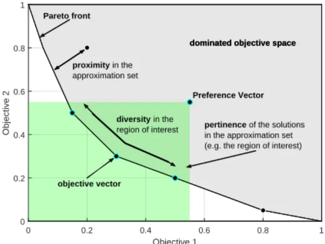
This approximation is a set of candidate solutions that represent the theoretical Pareto set. The features that describe the quality of an approximated Pareto set have been theorised in [67]. These features are:
• Proximity: The detected approximated Pareto set is desired to be as close as possible to the true Pareto-optimal front. Unfortunately, prox-imity cannot be used as a measure of quality of the approximation set during the optimisa-tion process, because the true Pareto set is not known (otherwise the problem would already be solved).
• Diversity: The desired approximation set should be uniformly distributed across the trade-off surface of the problem. This characterises the distribution of the approximation set both in the extent and uniformity of that distribution.
• Pertinence: Ideally, the approximation set should contain a number of solutions which are within some area (namely region of interest, see be-low) of the objective space. With this feature, the selection of a candidate solution from an approximation set becomes less complicated.
A representation of the desired features of an ap-proximation set are graphically represented in the two-objective case in Fig. 1, see [72].
With reference to the Pertinence of an approxi-mation set, the process of performing the selection of the solution among the available candidate solutions is named Decision Making. The criterion or algorithm that leads to the decision making is said to be the De-cision Maker (DM). In other words, the DM implic-itly classifies ‘interesting and uninteresting’ solutions. The area of the objective space where the interesting solutions fall within is named the Region Of Interest (ROI).
In summary, the solution of a multi-objective optimisation problem can be interpreted as a two-stage process: during the first two-stage the multi-objective
Objective 1 0 0.2 0.4 0.6 0.8 1 Objective 2 0 0.2 0.4 0.6 0.8 1 objective vector Preference Vector
pertinence of the solutions
in the approximation set (e.g. the region of interest)
proximity in the
approximation set
dominated objective space
diversity in the
region of interest
dominated objective space Pareto front
Figure 1. Proximity, diversity, and pertinence characteristics in an approximation set in two-objective space.
optimisation algorithm detects the approximation set while the DM performs the selection of the interest-ing solution from the approximation set in the second stage.
During both the stages, the main difficulty of the problem is the comparison and selection of solutions. Since one solution can outperform another solution with respect to one objective and not with respect to another (the solutions do not dominate each other), the selection of a set of solutions from a larger set is a chal-lenging task. This task becomes progressively more challenging as the number of objectives increases, see [25].
1.1. Multi-objective optimisation with more than three objectives: related work
The objectives of a multi-objective problem span a multi-dimensional space, namely the objective space. The size of the objective space grows exponentially with the number of objectives. This is analogous to the effect of dimensionality on the search space: for ex-ample a problem with 1000 variables is much harder (and not just twice) than a problem in 500 variables. A high-dimensional objective space is very hard to han-dle when a pairwise comparison is performed. Thus, the difficulty of a multi-objective problem grows ex-ponentially with the dimensionality of the objective space.
A multi-objective optimisation problem with more than three objectives is often referred to as a
many-objectiveoptimisation problem [25, 40, 58]. The study of this class of problem as well as the algorithms de-signed to tackle the difficulties dictated by a high-dimensional objective space are emerging research trends in literature. The main challenges have been highlighted in several articles, see e.g. [13, 14, 40]. These difficulties are detailed in the following list:
• The difficulty of performing pairwise compar-isons with the aim of selecting a set (a new population) increases with the number of ob-jectives, as it is likely that almost all candidate solutions within a population do not dominate each other, see [27, 52, 68].
• As a consequence of the dimensionality of the objective space, the number of candidate solu-tions required to produce an approximation set increases exponentially with the number of ob-jectives, see [37, 46].
• With the increase in the number of objectives, the computational cost of existing search oper-ators becomes infeasible [37].
• When the number of objectives increase, the number of generations required to produce an approximation set also increases exponentially.
• The increase in the number of objectives makes the problem less intuitive. Approaches which rely on spatial information between solutions in the objective space become ineffective. Fur-thermore, the visualisation of candidate solu-tions becomes difficult, often resulting in the use of heat-maps or parallel-coordinate plots. This poses a difficulty to the DM as the selec-tion of a final candidate soluselec-tion may become non-intuitive [86].
As a consequence, popular algorithms that per-form well on multi-objective optimisation with two or three objectives [15, 20, 82] display poor perfor-mance when applied to a problem that has many ob-jectives, e.g. five, see [33, 34, 39]. Studies on specific problems confirmed this fact [2, 44] while other arti-cles have observed this phenomenon with the aim of proposing methods for tackling a high number of ob-jectives [48, 68, 103] such as an objective space re-duction by the inclusion of the preferences within the search [61].
Therefore, several alternative algorithmic solu-tions have been proposed to tackle the difficulties
posed by a large number of objectives. An interesting example is the Non-dominated Sorted Genetic Algo-rithm III (NSGA-III), see [19, 43] based on the pre-vious NSGA-II. In this case, the dominance selection is revisited and adapted to the many-objective case by the use of structured weights (reference-points), in or-der to maintain high diversity throughout the optimi-sation process. This approach is similar to that taken in the Multi-Objective Evolutionary Algorithm based on Decomposition (MOEA/D) introduced in [95] to address the same difficulty, such that both NSGA-III and MOEA/D can be initialised with the same set of weights. Another feature of NSGA-III and MOEA/D is the use of niching during the selection of parent solutions for the recombination stage. This mecha-nism has been proposed to increase the exploitation of the algorithm. A further development of the MOEA/D idea has been presented in [96] where the MOAE/D with Dynamic Resource Allocation (MOEA/D-DRA) has been introduced. This MOEA/D-DRA decom-poses the many-objective space into many single-objective spaces (sub-problems) and then assigns different computational budgets to the various sub-problems. This algorithm, which has been a compe-tition winner at IEEE CEC [97] is currently one of the most effective solutions to tackle many-objective problems.
In [99] an acceleration of the search is achieved by biasing it: the direction of the knee points of the Pareto set (those points which represent the lack of a clear preference towards a specific objective) is pre-ferred. This approach shares with [98] the philosophy of avoiding extensive pairwise comparisons and han-dling large objective spaces better. Furthermore, this approach can be seen as a modern re-interpretation of a weighted sum approach where each weight coefficient is set to 1.
In [10, 11] the reference vector, i.e. a vector con-taining the preference weights for each objective, is integrated within the selection process in order to ex-clude solutions which do not fall within the ROI from the search. The idea of the incorporation of DM prefer-ences into the algorithmic selection has been proposed in other contexts, e.g. [60, 70, 71].
Over the past decade, the use of some metrics to measure the quality of non-dominated solution sets, namely performance indicators, have been introduced
to effectively perform the selection of solutions in the presence of many objectives. For example, the Indica-tor Based Evolutionary Algorithms (IBEAs) [41, 100, 102] use performance indicators as a method of intro-ducing selection pressure in place of dominance based selection, such as [21]. Amongst these indicators the hypervolume indicator, see e.g. [28], is a very power-ful approach which can lead to high performance re-sults.
The hypervolume indicator measures how much of the objective space is dominated by an approx-imation set. The way the hypervolume indicator is constructed is very appealing in real-world problems as it requires no information regarding the theoreti-cal Pareto-front (which is often unknown in practise.). Furthermore, the hypervolume indicator encompasses within it the information about proximity, diversity, and pertinence, ultimately evaluating the quality of the approximation set, see [31]. Successful examples of incorporating the hypervolume indicator into the op-timisation process during the selection stage can be found in [22] and [3], where an adapted version of the hypervolume indicator, named the contributing hyper-volume indicator, is used. Other successful cases of the hypervolume indicator being used during the selection process are given in [36] and [85] within the context of the Multi-Objective Covariance Matrix Adaptive Evo-lution Strategy (MO-CMA-ES).
Although hypervolume indicator is a very valu-able sorting criterion for selection, its calculation presents the drawback that it depends exponentially on number of objectives and becomes infeasible in many-objective problems. For this reason several papers at-tempted to propose algorithms for a fast calculation of the hypervolume indicator.
In [91] an algorithm based on a set theory of union and intersection of sets is proposed to calculate the hypervolume. The method proposed in [26] calculates the hypervolume as the sum of contribution given by the volume dominated by each solution, one by one. The latter method has been used to perform selec-tion within an Evoluselec-tionary Multi-Objective (EMO) algorithm in [50] which still resulted in being compu-tationally onerous. Several approximated calculations for the hypervolume indicator have been proposed, see e.g. [24]. In [88], the complexity of the hypervolume indicator is reduced by considering the objectives one
by one. In [3], the hypervolume indicator is approxi-mated by means of a Monte Carlo simulator.
1.2. Proposal of this article
While selection processes based on hypervolume in-dicators can be integrated in all meta-heuristics, not all the frameworks would be equally suitable to their embedding and their simplified calculation. Based on this consideration, this paper proposes a novel meta-heuristic for multi-objective optimisation which inte-grates a novel hypervolume indicator based selection process within the Pareto Archived Evolution Strat-egy (PAES) [51]. The latter is an algorithm that per-forms the selection of the individuals by grouping the solutions into sub-regions of the objective space. This mechanism is named the Adaptive Grid Algo-rithm (AGA). The resulting algoAlgo-rithm, namely the Co-variance Matrix Adaptation Pareto Archived Evolu-tion Strategy with Hypervolume-sorted Adaptive Grid Algorithm (CMA-PAES-HAGA) makes use of the search logic of the Covariance Matrix Adaptation Evo-lution Strategy (CMAES) [30] and the archive of the PAES structure. A preliminary version of the proposed algorithm without the newly proposed selection mech-anism has been proposed in [72], however, its prim-itive selection mechanism restricts its application to two-objective problems only.
CMA-PAES-HAGA proposes an algorithm for multi-objective optimisation which is specifically suited for four or more objectives.
The remainder of this article is organised in the following way. Section 2 introduces the notation and describes the proposed CMA-PAES-HAGA. Further-more, Section 2 provides the reader with the motiva-tion behind CMA-PAES-HAGA and emphasizes the differences with respect to its predecessor. Section 3 tests the proposed algorithm and compares it against the state-of-the-art and competition winning algorithm MOEA/D-DRA. This comparison is carried out over a set of test problems and over a real-world multi-objective problem with seven multi-objectives concerning an aircraft control system. Finally, Section 4 presents the conclusion to this work.
2. Covariance Matrix Adaptation Pareto Archived Evolution Strategy with
Hypervolume-sorted Adaptive Grid Algorithm
Covariance Matrix Adaptation (CMA) is a powerful approach to parameter variation which has demon-strated promising results in the optimisation of single-objective problems with CMA-ES [36], and multi-objective problems with MO-ES [85] and CMA-PAES [72]. These optimisation algorithms rely on CMA entirely for the variation of solution parameters, and therefore they do not suffer from the curse of di-mensionality which affects many optimisation algo-rithms which rely on reproduction operators. CMA-PAES is a multi-objective evolution strategy which first incorporated the CMA approach to variation with an adaptive grid scheme and Pareto archive. However, when moving to the optimisation of problems consist-ing of many (greater than three) objectives, it is the se-lection operators employed by these algorithms which render them ineffective or computationally infeasi-ble. The algorithm which is introduced in this section, named CMA-PAES-HAGA, proposes an approach to optimisation which is suitable for problems consisting of many objectives.
The approach to selection employed by MO-CMA-ES relies on the Contributing Hypervolume In-dicator (CHV) as a second-level sorting criterion, the calculation of which increases significantly with the number of objectives considered. In contrast, the ap-proach to selection employed by CMA-PAES is driven by an AGA which incurs little algorithm overhead in its calculation [72]. This AGA becomes ineffective when applied to many-objective problems as the num-ber of grid divisions which controls the division of the objective space and the size of the sub-populations be-comes increasingly sensitive with each additional ob-jective [70].
Whilst CMA-PAES has shown promising results in comparison to PAES, NSGA-II, and MO-CMA-ES [70, 72], it suffers from the curse of dimensionality when moving to many-objective problems.
This is because the process of the AGA for diver-sity preservation was designed with the two-objective case in mind. The grid location was stored as a scalar value starting at one, meaning it was not possible to use auxiliary information e.g. how close one
maxi-mally populated grid location was to another. This in-formation is beneficial when deciding which grid pop-ulation, from many which are maximally populated, will be selected for solution replacement when the archive is at capacity. The original AGA in CMA-PAES also replaced a solution at random, this ap-proach does not cause a significantly negative impact on its performance in the two-objective case, when configured with the recommended high number of grid divisions. However, when moving to problems con-sisting of a high number of objectives, a smaller num-ber of grid divisions must be selected, and a more so-phisticated approach to solution replacement must be considered.
CMA-PAES-HAGA is an Evolutionary Multi-objective Optimisation (EMO) algorithm, but more specifically, it is an evolution strategy for solving op-timisation problems consisting of many objectives. CMA-PAES-HAGA achieves many-objective optimi-sation by: 1) employing CMA for variation and opt-ing out of the use of reproduction operators; 2) em-ploying a new approach to selection in the form of a hypervolume-sorted AGA.
The following section begins by introducing the notation used throughout the paper, followed by a description of the CMA-PAES-HAGA algorithm in-cluding pseudo-code, mathematical procedures, and worked-through examples of the operators. The sec-tion concludes by defining the variants of CMA-PAES-HAGA and how they are implemented.
2.1. Notation and Data Structures
With the aim of defining the notation and data-structures used throughout this paper, M defines the number of objectives, N defines the population size, and a solution is defined by the tuple:
Xn,Vn,p¯succ,n,σn,σn∗,pn,c,Cn
(1)
whereXnandVnare pointers to a solution’s objective values and decision variables respectively.X is anM
byNmatrix of the entriesxmn, where every entryxmn refers to a solution’s objective value:
Xn=hx1n,x2n, . . . ,xMni (2) Similarly,V is anIbyNmatrix of the entriesvin, where every entryvin refers to a solution’s decision variable:
Vn=hv1n,v2n, . . . ,vIni (3) An objective function is required to evaluate the performance of candidate solutions (i.e. those solu-tions that could be the optimum). There can existM
objective functions with the definition in (4), these objective functions can be either minimised or max-imised.
f(Vn) = (f1(v),f2(v),f3(v), . . . ,fM(v)) (4)
A multi-objective optimisation problem in its gen-eral form can be described as:
optimise fm(v), m=1,2, . . . ,M; sub ject to gj(v)≥0, j=1,2, . . . ,J; hk(v) =0, k=1,2, . . . ,K; vi(L)≤vi≤vi(U)i=1,2, . . . ,I; (5)
The constraint functionsgj(v)andhk(v)impose inequality and equality constraints that must be satis-fied by a solutionvin order for it to be considered a feasible solution. Another condition which affects the feasibility of a solution, regards the adherence of a so-lutionv to values between the lower v(iL) and upper
v(iU)boundaries. The set containing all the feasible so-lutions is referred to as the decision space. The corre-sponding set of the values that each feasible solution can take is referred to as the objective space.
Each solution tuple also includes parameters used by the CMA variation operator, where ¯psucc,n∈[0,1] is the smoothed success probability, σn∈R+0 is the global step size,σnis the previous generation’s global step size, pn,c∈Rnis the cumulative evolution path, andCn∈Rv×vis the covariance matrix of the search distribution.
2.2. Algorithm design
The CMA-PAES-HAGA process outlined in Algo-rithm 1 begins by initialising algoAlgo-rithm parameters and randomly sampling the search-space to generate an initial parent populationXof sizeµ, the objective val-ues of each parent solution are then resolved using an objective function.X is anM byN matrix of entries
xmn, where everyxmn refers to a solution’s objective value, and Xnrefers to a solution (3).
Algorithm 1CMA-PAES-HAGA execution cycle 1: g←0
2: E← hε1=0,ε2=0, . . . ,εM=0i 3: initialise parent populationX,V
4: whiletermination criteria not metdo
5: forn=1, ...,λ do 6: Vn0←Vn 7: Vn0←Vn0+σn·N (0,Cn) 8: ifv(iL)v0inv(iU)then 9: v0in= ( v(iU) ifv0in>v(iU) v(iL) otherwise 10: end if 11: end for 12: Xn0 ←f(Vn0) 13: X∗=X∪X0 14: form=1, ...,Mdo 15: εm= ( x∗mn ifx∗mn>εm εm otherwise 16: end for 17: X,V←HypervolumeSortedAGA(X∗,E) 18: CMAParameterUpdate() 19: g←g+1 20: end while
The global CMA parameters are: the target suc-cess probability ptargetsucc , success threshold pthresh, step size damping d, step size learning ratecp, evolution path learning ratecc, and the covariance matrix learn-ing rateccov. The values for these parameters are set according to the parameters proposed in [36] where
ptargetsucc = (5+ p
1/2)−1, pthresh=0.44,d=1+n/2,
cp=ptargetsucc / 2+ptargetsucc ,cc=2/(n+2), andccov= 2/(n2+6).
With the initial parent population ready, the gen-erational loop begins:
Algorithm 2CMAParameterUpdate() 1: forn=1, ...,µdo
2: ifp¯0succ,n<pthreshthen 3: p0c,n← (1−cc)p 0 c,n+ p cc(2−cc)·σn∗ 4: C0n←(1−ccov)C 0 n+ccovp 0 c,np 0T c,n 5: else 6: p0c,n←(1−cc)p 0 c,n 7: C0n←(1−ccov)C 0 n +ccov p0c,np0Tc,n+cc(2−cc)C 0 n 8: end if 9: p¯in ←(1−cp)p¯in+cp·Xsucc 10: σin←σinexp 1 d ¯
psucc,in−ptargetsucc
1−ptargetsucc
11: end for
• The termination criterion is checked to de-cide whether the EMO process is terminated. In CMA-PAES-HAGA, the default condition for termination depends on reaching a maxi-mum number of function evaluations (specified
a priori).
• The offspring populationX0 of sizeλ is then generated using the parent population X and the CMA operator for variance.
• The offspring population’s solutions are then evaluated using an objective function, this ulation is then merged with the parent pop-ulation to create the intermediate poppop-ulation
X∗=X∪X0.
• The extreme values εm encountered for each objective during the optimisation process are then updated by checking if any objective value
x∗mn is higher than a corresponding stored ex-treme objective valueεm, and if so, replacing it. εm= ( x∗mn ifx∗mn>εm εm otherwise (6)
whereE is a vector containing all of the ex-treme values encountered for each objective.
E=hε1,ε2, . . . ,εMi (7)
• The intermediate population X∗ is then sub-jected to the hypervolume-sorted AGA selec-tion mechanism described in Secselec-tion 2.3. The mechanism will return a new parent population of sizeµwhich are considered to offer the best coverage of the objective space.
• The parameters used for the CMA operator for variance are then updated according to Algo-rithm 2. The solutions are considered success-ful (and marked as Xsucc=1) if they make it from the intermediate populationX∗to the par-ent population for the next generation. Con-versely, the solutions are considered unsuc-cessful (and marked asXsucc=0) if they are not transferred to the following generation and are not retained.
• The optimisation process then continues to the next generational iteration.
2.3. Hypervolume-sorted Adaptive Grid Algorithm
CMA-PAES-HAGA employs the Hypervolume-sorted AGA (HAGA) to select solutions to form the parent population for the next generation of the optimisation process. HAGA is a two-phase approach to selection, with the aim of being computationally feasible in the presence of many objectives. HAGA incorporates the use of a novel AGA implementation containing a num-ber of features in order to make the AGA implemen-tation suitable for many-objective optimisation. These features consist of:
• A new data structure for storing a solution’s grid number up to any number of objectives;
• A new grid-proximity method for grid selection when searching for a solution to remove;
• A new scheme for the maintenance of global extremes for objectives.
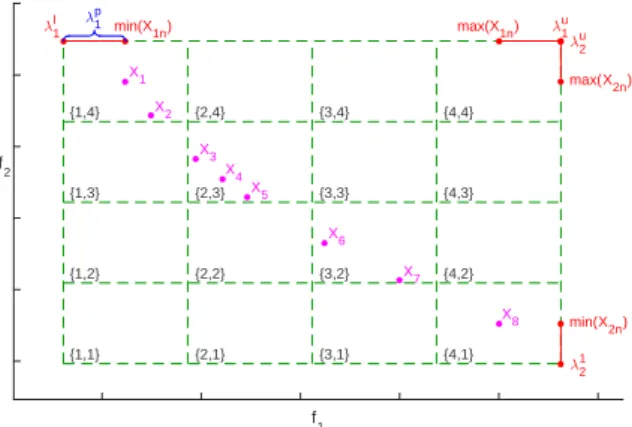
HAGA aims to use a two-phase approach to re-duce the number of solutions which are to be con-sidered by the narrow-phase, through the use of a broad-phase. The grid structure when visualised for a two-objective approimation set can be seen in Fig-ure 2, where the grid squares have been indicated with dashed lines, and the grid locations have been indi-cated with vectors surrounded by braces. In this ex-ample, the grid location{2,3}refers to a grid square
which defines a grid population consisting of the solu-tionsX3,X4andX5.
This is achieved by mean of the execution life-cycle listed in Algorithm 3, whereXis an approxima-tion set of soluapproxima-tionsXn,Ais the archive of parent solu-tions selected by HAGA,Γis a grid location consisting
of multiple solutions, andµandλ are the number of parent and offspring solutions respectively.CHVΓt is
a vector of entries resulting from the execution of the contributing hypervolume indicator on the solutions in the grid populationΓt, such that min(CHVΓt)would
yield the solution which offers the lowest explicit hy-pervolume indicator contribution in regards to the ob-served grid population.
Algorithm 3HypervolumeSortedAGA(X,λ,µ) 1: forn = 1 :λ do 2: if|A|<µthen 3: A←A∪Xn 4: else 5: Γt←ClosestGridFromMaxPopulated(Γn) 6: Γt←Γt∪Xn 7: CHVΓt ←ContributingHV(Γt) 8: ifmin(CHVΓt) =Xnthen
9: Discard candidate solution
10: else
11: Discard min(CHVΓt)solution
12: A←A∪Xn
13: end if
14: end if
15: end for returnA
In Algorithm 3, Line 5 identifies the grid loca-tion closest to the candidate soluloca-tion and resolves a grid population. This is considered the broad-phase of the two-phase approach. Once a grid location has been identified, it is used in the calculation of the narrow-phase (Line 7), which depends on the contributing hy-pervolume indicator described in the following.
The basic principle of HAGA is to benefit from the CHV algorithm’s ability to discriminate solutions based on the explicit hypervolume they contribute to a population, but to do so in a way that doesn’t in-troduce the computational infeasibility of using CHV on populations consisting of many-objective solutions. HAGA achieves this through the use of the adaptive
grid, where the objective space covered by a popula-tion is divided into a grid consisting of grid areas. This grid has a capacity for the number of solutions it can store, this capacity is set to µ, which is the number of parent solutions desired for selection. The solutions within the intermediate population (the parent and off-spring population) are then added to this grid one by one. Throughout this process, there is no computation of the CHV algorithm until the grid reaches capac-ity, at which point the CHV is only computed at grid area level. This ensures that the CHV is computed for only a small number of solutions, in order to determine which solution is to be evicted from the grid area to prevent the grid from exceeding capacity. In contrast, the CHV algorithm simply computes the CHV indica-tor value for every solution in the population.
The CHV indicator can be calculated by first cal-culating the hypervolume indicator quality XHV of a populationX: HV fre f,X = Λ [ Xn∈X h f1(Xn),f1re f i × · · · × fm(Xn),fmre f ! (8)
where fmre f is the reference point for objectivem, andXmis a set of objective values for objectivemfrom the current population.
With the hypervolume indicator quality of the population calculated, it is possible to calculate the CHV indicator value of each candidate solution within the population. For each solution in the population, the solution is first removed from the population to form the temporary populationXT, and then the hypervol-ume indicator qualityXHVT is calculated for this tempo-rary population. The CHV indicator value is then cal-culated by subtractingXHVT fromXT, this is the explicit hypervolume contribution of the candidate solution. Once the CHV indicator value has been calculated for every candidate solution, it is possible to order them by descending value so that they are ordered by the greatest explicit hypervolume indicator contribution. The firstµsolutions are then selected to form the next parent population. This approach has been listed in Al-gorithm 4, whereX is a set of solutions from a grid population.
Algorithm 4Contributing Hypervolume Indicator ex-ecution life-cycle ContributingHV(fre f,X) 1: XHV←HV(fre f,X) 2: forn = 1 :λ do 3: Xt←X\Xn 4: HVn←HV(fre f,Xt) 5: CHVn←XHV−HVn 6: end for returnCHV
It must be noted that the purpose of HAGA is to return a set of solutions which is of sizeµ, this size parameter must be defined before the execution of the algorithm. The µ size parameter is used within the HAGA selection approach, and as such the output set is dependent on its definition. This is unlike the CHV selection approach, which will return a set of hyper-volume indicator values for each solution in the set on which it was executed.
The process for HAGA in its entirety is mathe-matically described herein.∆ defines the number of desired grid divisions for an objective within the ob-jective space.Γis anMbyNmatrix of entriesγmn,
Γn=hγ1n,γ2n, . . . ,γMni (9) whereΓnrefers to a row in theΓmatrix, and every
en-tryγmnrefers to the grid location of an objective value
xmnin the divided objective space.
To calculateΓn, the grid locationγmnof each ob-jective value xmn for each solution Xn needs to be resolved. To calculate a solution’s grid location, the padded grid lengthΛ
Λ=hλ1,λ2, . . . ,λMi (10) for each objective needs to be calculated using the low-est and highlow-est objective value for each objective in the population: f1 f 2 {1,1} {2,1} {3,1} {4,1} {1,2} {2,2} {3,2} {4,2} {1,3} {2,3} {3,3} {4,3} {1,4} {2,4} {3,4} {4,4} X1 X2 X3 X4 X5 X6 X7 X8 61l 6 1 u min(X1n) max(X1n) 621 62u min(X2n) max(X2n) 61p
Figure 2. Visualisation of the AGA and its elements on a two-ob-jective problem with four grid divisions. Vectors within braces indi-cate the grid location.
λmp=|min(Xm)−max(Xm)| 2(∆−1) λml =min(Xm)−λmp λmu=max(Xm) +λmp λm=|λml −λmu| (11)
whereλml is the start point of the grid for objectivemin the objective space, andλmuis the end point of the grid for objectivemin the objective space. These elements have been illustrated in Figure 2.
With the grid length and range calculated, it is possible to get the grid location of each solution’s ob-jective value using:
γmn= & xmn−λml λm ∆ ' (12)
When the entries of Γn have been calculated, it can be used to identify the grid location of a solution
Xn. In this new method, the grid locationΓnis defined by a vector rather than a scalar, for example in a five-objective problem a grid location can be described by being at locationΓn=h2,4,1,1,2i.
As an example, a population X of five (N=5)
solutionsXnfor a five-objective problem (M=5) has been presented in Table 1.
The population X has been subjected to the HAGA mechanism to resolve the grid locationΓn
vec-Table 1.An example populationXof objective valuesxmn to be
subjected to the HAGA mechanism.
x1n x2n x3n x4n x5n X1 0.5 0.5 5.0 2.5 1.5 X2 0.6 0 5.0 3.0 1.4 X3 0.5 3.5 4.5 2.5 1.5 X4 0.8 3.2 4.2 3.0 1.2 X5 1 3 4 2 1
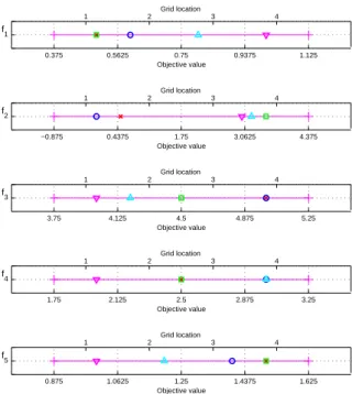
tor of each solutionXn, with an adaptive-grid config-uration of four grid divisions (∆=4). The grid loca-tions resolved by the HAGA mechanism have been presented in Table 2. In this example, each solution
Xn has been assigned to a grid location Γn, for ex-ample, solution X2 which consists of the objectives
h0.5,0.5,5.0,2.5,1.5ihas been assigned to the grid lo-cationh2,1,4,4,3i. The solution values for each ob-jectivexmnhave been plotted in their respective grid locationsγmin Figure 3.
Table 2.Grid locationsΓfor the example populationXof objective valuesxmn. γ1n γ2n γ3n γ4n γ5n Γ1 1 1 4 3 4 Γ2 2 1 4 4 3 Γ3 1 4 2 3 4 Γ4 3 4 2 4 2 Γ5 4 4 1 1 1
The results from this example show that the exam-ple population does not consist of any solutions which are in the same grid square (otherwise theirΓentries
would be identical).
The method for selecting a grid location to re-move a solution when the archive is at capacity is im-portant when moving to many-objective problems. Se-lecting at random from grid locations which are at the same population density increases the probability of causing genetic drift, and decreases the diversity qual-ity of the population. This undesirable effect is scaled exponentially as the number of objectives increase, and it is for this reason that many modern EMO algo-rithms now incorporate a niching approach when con-cerned with selection [19, 96]. Therefore, it is desir-able to find the grid location which is close to both so-lutions in the objective space and also at a higher den-sity. 0.375 0.5625 0.75 0.9375 1.125 f 1 Objective value 1 2 3 4 Grid location −0.875 0.4375 1.75 3.0625 4.375 f 2 Objective value 1 2 3 4 Grid location 3.75 4.125 4.5 4.875 5.25 f3 Objective value 1 2 3 4 Grid location 1.75 2.125 2.5 2.875 3.25 f4 Objective value 1 2 3 4 Grid location 0.875 1.0625 1.25 1.4375 1.625 f5 Objective value 1 2 3 4 Grid location
Figure 3. One dimensional plots illustrating the grid locations re-solved by the HAGA mechanism for each objective value.
Storing grid locations as a single scalar value is not helpful when calculating distance between grid locations or for storing grid locations for a many-objective problem. The grid location structure used in the proposed AGA scheme described above enables an intuitive method for finding the distance between grid locations. By establishing the grid location which a candidate solution would be assigned to if it was part of the archive, it is possible to find the difference be-tween its grid location and other grid locations which are at high density to find out which one it’s closest to by summing the difference of the grid location vectors.
For example, if a new solution
X6=h0.6,0.5,4,3,1.1i
was to be included as a candidate solution as part of the HAGA mechanism, it would resolve a grid loca-tion ofΓ6=h2,1,1,4,2i. The distanceδnbetween this grid location and the grid locations of the other solu-tions can be found by finding the absolute difference of each corresponding entry of the candidate solution’s grid location and another solution from the population, and then summing those values.
δn= N
∑
n=1|γm∗−γmn| (13)
The distancesδnbetween the grid locationΓ6of solutionX6and all the other solutions in the population presented in Table 1 have been presented in Table 3. The results show that the solution closest in proximity to solutionX6is solutionX2.
Table 3.Grid locationsΓfor the example populationXof objective valuesxmn.
Γ1 Γ2 Γ3 Γ4 Γ5
δ6 7 4 8 5 9
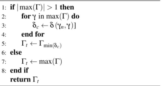
Using this method of resolving densely populated grid locations, which are closest in proximity to a can-didate solution, it is possible to implement the ap-proach listed in Algorithm 5.
Algorithm 5ClosestGridFromMaxPopulated(Γn) 1: if|max(Γ)|>1then 2: forγin max(Γ)do 3: δc←δ(γn,γ)] 4: end for 5: Γt←Γmin(δc) 6: else 7: Γt←max(Γ) 8: end if returnΓt
This algorithm is invoked by Line 5 of Algorithm 3 byClosestGridFromMaximallyPopulated(Xn). Line 1 checks to see if there is a single grid location which contains the most solutions, if there is more than one grid location that contains the most number of so-lutions then the algorithm identifies the grid square which is closest in proximity to the candidate solu-tion.δncrefers to the difference between the candidate solution’s grid location and other grid locations, and
Γmin(δc) refers to the grid location which is the
clos-est in proximity among those containing the maximal number of solutions.
In previous AGA implementations, the extreme values for each objective were preserved at grid level. In the proposed AGA scheme, solutions containing
ex-treme values for objectives (with the candidate solu-tion taken into considerasolu-tion) are removed from the population before it is subjected to the AGA. No special treatment is given to solutions containing lo-cally (within their grid location) extreme objective val-ues. This ensures candidate solutions are given a bet-ter chance of enbet-tering the archive than they would have had if they had come up against those solutions containing extreme values. This preserves the overall spread whilst encouraging new solutions to enter the archive.
3. Numerical Results
In order to test the proposed CMA-PAES-HAGA scal-able WFG multi-objective test suite proposed in [32] has been considered in five, seven and ten objectives where each objective had 24 variables.
The proposed CMA-PAES-HAGA has been run with a parent population of size µ=100 individuals, archive capacity of 100 individuals, number of grid di-visions equal to 3. The chosen value of 3 has been set subsequent to a tuning where the values between 2 and 20 have been taken into consideration. The 3 setting has been chosen as it proved to give the best perfor-mance in terms of computational cost. A lower value of grid divisions would result in fewer grid squares and therefore larger grid square populations. This will result in worst performance in the computation of the CHV indicator which is used at grid level. In con-trast, higher numbers of grid divisions will result in many more grid locations which may hold only a few solutions and often only a single solution. This sce-nario does not ensure the best performance out of the CHV indicator, as often only a single solution will be in each grid square. The CMA-PAES-HAGA al-gorithm has been compared with MOEA/D-DRA [96] with both µ and λ populations of 100 individuals, niche size of 20, and maximum update number equal to 2. A population size of 100, in combination with the number of grid divisions set to 3, prevents the com-putationally infeasible scenario where a large number of solutions are considered when calculating the hy-pervolume indicator values. Both algorithms consid-ered in the pairwise comparisons use diversity opera-tors in order to offer a well-distributed representation
of the trade-off surface for each problem, with CMA-PAES-HAGA using the hypervolume indicator driven approach, and MOEA/D-DRA using the weighted ap-proach. Both the algorithms have been run for 50,000 function evaluations. Each algorithm for each problem has been run 30 times. The choice of this algorithm has been made considering that this is currently one of the algorithms which displayed the best performance on five-objective problems, see [70].
All test cases have been executed on a desktop computer with the configuration listed in Table 4.
Table 4. Hardware and software configurations of the computer used to generate the results.
Configuration name Configuration value
Architecture Linux-x64
RAM 16 GB
CPU Intel(R) Xeon(R) CPU E5-1620 v2
@ 3.70GHz Total CPU Cores 4
MATLAB version R2014a 64-bit (glnxa64) Hypervolume Indicator WFG HV 1.0.3
In order to evaluate the performance the hypervol-ume indicator has been chosen by following the indi-cations in [31, 83]. The hypervolume indicator is se-lected because it is scaling independent and requires no prior knowledge of the true Pareto-optimal front, this is important when working with real-world prob-lems which have not yet been solved. The hypervol-ume indicator allows for a measurement as to which algorithm covers the greatest amount of the search space. A greater hypervolume indicator value indi-cates superior performance.
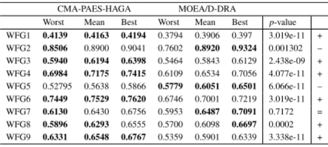
Tables 5, 6, and 7 show the hypervolume indica-tor on average and in the best and worst cases over the 30 runs available in the cases of five, seven and ten ob-jectives, respectively. The best results are indicated in bold for clarity. The hypervolume indicator values can only be compared within a specific test-case for each of the considered algorithms. For example, the results for CMA-PAES-HAGA on the five-objective WFG1 test-case are directly comparable to the correspond-ing MOEA/D-DRA results on the same row of Table 5. This is because each test case requires a reference point, which is formed by using the extreme values en-countered for each of the objectives in all of the 60
ap-proximation sets (30 runs for CMA-PAES-HAGA and 30 runs for MOEA/D-DRA).
In order to enhance the statistical significance of the results Wilcoxon test [89] has been performed. In each table, the p value as well as the result of the Wilcoxon tests are shown: a “+” indicates that the proposed CMA-PAES-HAGA statistically out-performed MOEA/D-DRA, a “-” indicates that the proposed MOEA/D-DRA statistically outperformed CMA-PAES-HAGA, while a “=” indicates that the al-gorithm statistically have the same performance.
Table 5. Hypervolume results from 30 executions of CMA-PAES-HAGA and MOEA/D-DRA on the WFG test suite with five objec-tives. The boldface values indicate superior performance
CMA-PAES-HAGA MOEA/D-DRA
Worst Mean Best Worst Mean Best p-value
WFG1 0.4139 0.4163 0.4194 0.3794 0.3906 0.397 3.019e-11 + WFG2 0.8506 0.8900 0.9041 0.7602 0.8920 0.9324 0.001302 – WFG3 0.5940 0.6194 0.6398 0.5464 0.5843 0.6129 2.438e-09 + WFG4 0.6984 0.7175 0.7415 0.6109 0.6534 0.7056 4.077e-11 + WFG5 0.52795 0.5638 0.5866 0.5779 0.6051 0.6501 6.066e-11 – WFG6 0.7449 0.7529 0.7620 0.6746 0.7001 0.7219 3.019e-11 + WFG7 0.6130 0.6430 0.6756 0.5953 0.6487 0.7091 0.7172 = WFG8 0.5896 0.6293 0.6555 0.5700 0.6098 0.6697 0.0002 + WFG9 0.6331 0.6548 0.6767 0.5359 0.5901 0.6339 3.338e-11 +
Table 6. Hypervolume results from 30 executions of CMA-PAES-HAGA and MOEA/D-DRA on the WFG test suite with seven ob-jectives. The boldface values indicate superior performance
CMA-PAES-HAGA MOEA/D-DRA
Worst Mean Best Worst Mean Best p-value
WFG1 0.3472 0.3509 0.3552 0.3191 0.3261 0.3348 3.019e-11 + WFG2 0.8555 0.8999 0.9272 0.7817 0.9285 0.9598 2.01e-08 – WFG3 0.5835 0.6048 0.6154 0.4917 0.5513 0.5936 4.0e-11 + WFG4 0.6834 0.7056 0.7247 0.5881 0.6509 0.7067 6.1e-10 + WFG5 0.4755 0.5281 0.5605 0.4775 0.5253 0.5823 0.3710 = WFG6 0.8484 0.8546 0.8592 0.8216 0.8326 0.8472 3.0e-11 + WFG7 0.6342 0.6829 0.7222 0.5957 0.6634 0.7392 0.0127 + WFG8 0.6245 0.6771 0.7188 0.6013 0.6671 0.7335 0.5011 = WFG9 0.5786 0.6231 0.6532 0.4302 0.5228 0.6312 1.95e-10 +
Table 7. Hypervolume results from 30 executions of CMA-PAES-HAGA and MOEA/D-DRA on the WFG test suite with ten objec-tives. The boldface values indicate superior performance.
CMA-PAES-HAGA MOEA/D-DRA
Worst Mean Best Worst Mean Best p-value
WFG1 0.2998 0.3045 0.3112 0.2713 0.2789 0.2910 3.019e-11 + WFG2 0.9397 0.9559 0.9656 0.9516 0.9719 0.9786 5.072e-10 – WFG3 0.6545 0.6609 0.6673 0.5315 0.5896 0.6260 3.012e-11 + WFG4 0.6744 0.7075 0.7679 0.6189 0.6990 0.765 0.3871 = WFG5 0.4658 0.4927 0.5127 0.4064 0.4522 0.5040 1.856e-09 + WFG6 0.6314 0.6430 0.6679 0.5458 0.5694 0.5981 3.019e-11 + WFG7 0.6727 0.7250 0.8051 0.5841 0.6627 0.7738 2.377e-07 + WFG8 0.5742 0.5988 0.6341 0.4698 0.5827 0.6813 0.3112 = WFG9 0.5444 0.6046 0.6348 0.3673 0.4414 0.5574 3.689e-11 +
It must be remarked that the calculation of the hypervolume indicator is, albeit a very reliable mea-sure, computationally extremely onerous when more than three objectives are considered [6]. The calcu-lation of a single hypervolume indicator value for a ten-objective approximation set can in some cases, re-quire up to twelve hours with the hardware configu-ration specified in Table 4. For this reason we had to limit this comparison to only two algorithms. On the other hand we know from the literature, see e.g. [96], that MOEA/D-DRA outperforms many popular multi-objective optimisation algorithms on this test-suite.
Numerical results show that in the five-objective case, CMA-PAES-HAGA outperforms MOEA/D-DRA since the proposed algorithm displays a better perfor-mance for six problems and is outperformed in two cases. In the seven and ten objective cases, the per-formance of CMA-PAES-HAGA is clearly superior to that of MOEA/D-DRA. The proposed CMA-PAES-HAGA significantly outperforms MOEA/D-DRA for six problems and is outperformed in only one case, that is WFG2 where the performance of MOEA/D-DRA appears to be quite good. Although there is no general rigorous proof for the No Free Lunch Theo-rem for multi-objective optimisation [17, 90] the per-formance of multi-objective algorithms is also prob-lem dependent.
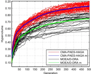
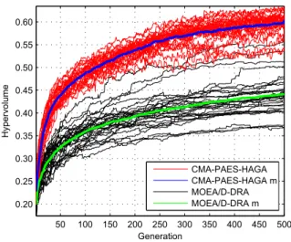
Fig. 4, 5, and 6, show the variation in the hyper-volume value of the algorithmic generations in five, seven, and ten objectives, respectively, in the case of WFG9. In each figure the hypervolume values associ-ated to individual and average runs are highlighted.
Results in the figures clearly show how the perfor-mance of the proposed CMA-PAES-HAGA improves with the increase of the number of objectives with respect to the performance of MOEA/D-DRA. This trend is evident for WFG9 but is also generally true for the other test problems.
3.1. Multi-objective Optimisation of Aircraft Control System Design
An important engineering problem, here used as an application example, is the design of a fighter air-craft control system. This, as well as many engineering problems, are naturally multi-objective as engineers desire that multiple objectives are simultaneously
op-50 100 150 200 250 300 350 400 450 500 0.20 0.25 0.30 0.35 0.40 0.45 0.50 0.55 0.60 Generation Hypervolume CMA-PAES-HAGA CMA-PAES-HAGA m MOEA/D-DRA MOEA/D-DRA m
Figure 4. Evolution of the hypervolume indicator results (single runs and mean values m) for five-objective WFG9 test case.
50 100 150 200 250 300 350 400 450 500 0.10 0.20 0.30 0.40 0.50 0.60 0.70 0.80 0.10 0.20 Generation Hypervolume CMA-PAES-HAGA CMA-PAES-HAGA m MOEA/D-DRA MOEA/D-DRA m
Figure 5. Evolution of the hypervolume indicator results (single runs and mean values m) for seven-objective WFG9 test case.
timised. Figure 7 presents an illustration of an air-craft with the three main axes of motion labelled: the Roll (longitudinal) axis, the Pitch (lateral) axis, and the Yaw (vertical) axis. A combination of changes are made to both the angles and the rates of the angular velocities during the motion of the aircraft [80].
The system and input data for the fighter aircraft in this problem have been listed in the following:
50 100 150 200 250 300 350 400 450 500 0.20 0.25 0.30 0.35 0.40 0.45 0.50 0.55 0.60 Generation Hypervolume CMA-PAES-HAGA CMA-PAES-HAGA m MOEA/D-DRA MOEA/D-DRA m
Figure 6. Evolution of the hypervolume indicator results (single runs and mean values m) for ten-objective WFG9 test case.
Figure 7.The three main axes of an Aircraft body.
A= −0.2842 −0.9879 0.1547 0.0204 10.8574 −0.5504−0.2896 0.0000 −199.8942−0.4840−1.6025 0.0000 0.0000 0.1566 1.0000 0.0000 B= 0.0000 0.0524 0.4198 −12.7393 50.5756 21.6753 0.0000 0.0000
These matrices represent the system state of the vehicle and are used in the control vector. More specif-ically, matrixAis the kinetic energy matrix whileBis the Coriolis matrix, see [80] for details. Then,
u=Cup+Kx (14)
whereupis the pilot’s control input vector:[16,0].
The seven problem variables k1 tok7 form part of the state space gain matrices, these represent gains applied to the various signals involved in the fighter aircraft control system:
C= 1 0 k51 ;K= k6k1k20 k7k3k40 . (15)
The optimisation problem studied in this example consists of finding the values of the gain coefficients
[k1,k2,k3,k4,k5,k6,k7] such that the following seven objectives are simultaneously minimised:
1. The spiral root.
2. The damping in roll root. 3. The dutch-roll damping ratio. 4. The dutch-roll frequency. 5. The bank angle at 1.0 seconds. 6. The bank angle at 2.8 seconds. 7. The control effort.
Objectives 1 to 4 are the eigenvalues associated to the matrixA+BK, Objectives 5 and 6 are the bank angle taken at two intervals (1 s and 2.8 s) according to Military Specification [8] requirements, Objective 7 is the sum of squares of gain vector.
Further details regarding the aircraft dynamic model and the problem variables are available in [4, 23]. This optimisation problem will be referred to as Lateral Controller Synthesis (LATCON) herein.
The proposed CMA-PAES-HAGA has been tested to solve the LATCON problem and its performance has been compared with that of MOEA/D-DRA, NSGA-II, and a newly proposed algorithm for solving many-objective problems namelyθ-Dominance based Evolutionary Algorithm (θ-DEA) [92]. The parame-ter setting of CMA-PAES-HAGA and MOEA/D-DRA is the same mentioned above. NSGA-II was executed with µ andλ populations of 100 individuals, and a mutation rate of 1n wherenis the number of problem variables (seven in this case). The same population sizeµ=100 has been used also forθ-DEA. Each al-gorithm was given a limit of 10,000 function evalua-tions. The three competing algorithms have been cho-sen by considering that MOEA/D-DRA and θ-DEA are specialised algorithms for problems with many objectives, whilst NSGA-II is used here as a classic
benchmark algorithm. For each algorithm in this study 30 independent runs have been performed.
The hypervolume indicator was measured at each generation throughout the optimisation process. At the end of the optimisation the following hyper-volume indicator average values have been yielded: CMA-PAES-HAGA (3.5616e+37), MOEA/D-DRA (2.9182e+37), θ-DEA ( 2.3992e+37) and NSGA-II (2.3536e+36). These results clearly show that NSGA-II, albeit popular and efficient for two-objective and three-objective problems, does not offer good perfor-mance on this seven-objective problem as the corre-sponding hypervolume indicator value is one order of magnitude inferior than that associated to the other two algorithms.
The comparison between CMA-PAES-HAGA, MOEA/D-DRA, andθ-DEA show that although the latter two are good algorithms in multi-objective opti-misation for problems with more than three objectives, they are both outperformed by CMA-PAES-HAGA on this control engineering problem.
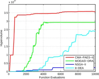
The evolution of the hypervolume indicator for the four algorithms under consideration has been plot-ted in Fig. 8. 0 2000 4000 6000 8000 10000 0 0.5 1 1.5 2 2.5 3 3.5 x 1037 Function Evaluations Hypervolume CMA−PAES−II MOEA/D−DRA NSGA−II θ−DEA
Figure 8. Evolution of the hypervolume indicator results for the seven-objective LATCON problem.
Fig. 8 highlights that NSGA-II is unsuitable to solve the LATCON problem. This result was expected as several studies show that NSGA-II displays poor performance in problems composed of more than three objectives, see e.g. [18]. In contrast, MOEA/D-DRA
appears to be well suited to address the LATCON problem. This result was also expected as it confirms the findings reported in [38] where it is shown how a MOEA/D scheme tends to perform much better than NSGA-II in many-objective problems.
The performance ofθ-DEA is also quite good for this problem. However, θ-DEA for this problem and for the given computational budget appears to display a performance which is not as good as that of CMA-PAES-HAGA and MOEA/D-DRA. Furthermore, from an analysis of the trend in Fig. 8, unlike MOEA/D-DRA,θ-DEA probably required a larger budget to de-tect better values of hypervolume (the trend appears still to grow at the end of the budget).
The comparison between CMA-PAES-HAGA and MOEA/D-DRA indicates that the proposed algo-rithm not only achieves better hypervolume indica-tor values at the end of the computational budget, but also is much faster than MOEA/D-DRA to reach a good hypervolume indicator value. It can be observed that, for the LATCON problem, CMA-PAES-HAGA achieves a good hypervolume value after only 10 gen-erations. This feature makes CMA-PAES-HAGA an interesting option for those problems which demand a solution in a short time or computationally expensive problems. Furthermore, it can be observed that at the end of the executions, while NSGA-II and MOEA/D-DRA appear to be incapable to enhance upon their corresponding hypervolume indicator value, CMA-PAES-HAGA is still able to obtain marginal improve-ments.
4. Conclusion
This article proposes a novel algorithm for multi-objective optimisation with four or more multi-objectives. The proposed algorithm contains a novel selection mechanism suitable to compare solutions consisting of many objectives. This selection mechanism makes use of an approximated hypervolume logic in order to se-lect solutions for the following generation. This selec-tion mechanism overcomes the limitaselec-tion of the true hypervolume indicator (selection by CHV) whose ap-plication would be computationally infeasible, whilst still resulting in an algorithm which is very efficient for multi-objective problems with more than four ob-jectives.
Numerical results show that the proposed CMA-PAES-HAGA framework displays an excellent perfor-mance in five, seven, and ten-objective optimisation problems when compared to MOEA/D-DRA which represents the state-of-the-art for many-objective op-timisation problems. Furthermore, a real-world seven-objective problem concerning the design of an aircraft control system is also used as a benchmark. In the latter case, it is evident that CMA-PAES-HAGA is a high-performance option, in terms of quickly achiev-ing a high hypervolume indicator value, when the problem is characterised by many conflicting objec-tives.
References
[1] H. Adeli and K. C. Sarma,Cost Optimization of Structures: Fuzzy Logic, Genetic Algorithms, and Parallel Computing. New York, NY, USA: John Wiley & Sons, Inc., 2006. [2] M. Antonelli, P. Ducange, and F. Marcelloni, “A fast and
efficient multi-objective evolutionary learning scheme for fuzzy rule-based classifiers,”Information Sciences, vol. 283, no. 0, pp. 36 – 54, 2014.
[3] J. Bader and E. Zitzler, “Hype: An algorithm for fast hypervolume-based many-objective optimization,” Evolu-tionary Computation, vol. 19, no. 1, pp. 45–76, 2011. [4] J. H. Blakelock,Automatic control of aircraft and missiles.
John Wiley & Sons, 1991.
[5] A. Bolourchi, S. F. Masri, and O. J. Aldraihem, “Stud-ies into computational intelligence and evolutionary ap-proaches for model-free identification of hysteretic sys-tems,”Computer-Aided Civil and Infrastructure Engineer-ing, vol. 30, no. 5, pp. 330–346, 2015. [Online]. Available: http://dx.doi.org/10.1111/mice.12126
[6] K. Bringmann, T. Friedrich, C. Igel, and T. Voß, “Speeding up many-objective optimization by monte carlo approxima-tions,”Artificial Intelligence, vol. 204, pp. 22–29, 2013. [7] A. Cerveira, J. Baptista, and E. J. S. Pires, “Wind farm
distri-bution network optimization,”Integrated Computer-Aided Engineering, vol. 23, no. 1, pp. 69–79, 2015.
[8] C. R. Chalk, T. Neal, T. Harris, F. E. Pritchard, and R. J. Woodcock, “Background information and user guide for mil-f-8785b (asg),’military specification-flying qualities of piloted airplanes’,” DTIC Document, Tech. Rep., 1969. [9] J. Cheng, G. Zhang, F. Caraffini, and F. Neri,
“Multicrite-ria adaptive differential evolution for global numerical opti-mization,”Integrated Computer-Aided Engineering, vol. 22, no. 2, pp. 103–107, 2015.
[10] R. Cheng, Y. Jin, M. Olhofer, and B. Sendhoff, “A reference vector guided evolutionary algorithm for many-objective optimization,”IEEE Transactions on Evolutionary Compu-tation, vol. PP, no. 99, pp. 1–1, 2016, to appear.
[11] R. Cheng, M. Olhofer, and Y. Jin, “Reference vector based a posteriori preference articulation for evolutionary multiob-jective optimization,” inEvolutionary Computation (CEC), 2015 IEEE Congress on, May 2015, pp. 939–946. [12] J. Y. J. Chow, “Activity-based travel scenario analysis with
routing problem reoptimization,”Computer-Aided Civil and Infrastructure Engineering, vol. 29, no. 2, pp. 91–106, 2014. [Online]. Available: http://dx.doi.org/10.1111/mice.12023 [13] C. A. C. Coello, “Evolutionary multi-objective
optimiza-tion: some current research trends and topics that remain to be explored,”Frontiers of Computer Science in China, vol. 3, no. 1, pp. 18–30, 2009.
[14] C. A. Coello Coello, “Research directions in evolution-ary multi-objective optimization,”Evolutionary Computa-tion Journal, vol. 3, no. 3, pp. 110–121, 2012.
[15] C. A. Coello Coello and G. B. Lamont, Applications of multi-objective evolutionary algorithms. World Scientific, 2004, vol. 1.
[16] L. Coletta, E. Hruschka, A. Acharya, and J. Ghosh, “Using metaheuristics to optimize the combination of classifier and cluster ensembles,”Integrated Computer-Aided Engineer-ing, vol. 22, no. 3, pp. 229–242, 2015.
[17] D. W. Corne and J. D. Knowles, “No free lunch and free left-overs theorems for multiobjective optimisation problems,” inEvolutionary Multi-Criterion Optimization. Springer, 2003, pp. 327–341.
[18] K. Deb and H. Jain, “Handling many-objective problems us-ing an improved nsga-ii procedure,” in2012 IEEE Congress on Evolutionary Computation, 2012, pp. 1–8.
[19] ——, “An evolutionary many-objective optimization algo-rithm using reference-point-based nondominated sorting ap-proach, part i: Solving problems with box constraints,” Evolutionary Computation, IEEE Transactions on, vol. 18, no. 4, pp. 577–601, Aug 2014.
[20] K. Deb, “Multi-objective optimization,”Multi-objective op-timization using evolutionary algorithms, pp. 13–46, 2001. [21] K. Deb, A. Pratap, S. Agarwal, and T. Meyarivan, “A fast
and elitist multiobjective genetic algorithm: Nsga-ii,” Evo-lutionary Computation, IEEE Transactions on, vol. 6, no. 2, pp. 182–197, 2002.
[22] M. Emmerich, N. Beume, and B. Naujoks, “An emo algorithm using the hypervolume measure as selection criterion,” in Evolutionary Multi-Criterion Optimization. Springer, 2005, pp. 62–76.
[23] B. Etkin,Dynamics of atmospheric flight. Courier Corpo-ration, 2012.
[24] R. M. Everson, J. E. Fieldsend, and S. Singh,Adaptive Com-puting in Design and Manufacture V. London: Springer London, 2002, ch. Full Elite Sets for Multi-objective Opti-misation, pp. 343–354.
[25] M. Farina and P. Amato, “On the optimal solution definition for many-criteria optimization problems,” inProceedings of the NAFIPS-FLINT International Conference, J. Keller and O. Nasraoui, Eds., 2002, pp. 233 – 238.
[26] M. Fleischer, Evolutionary Multi-Criterion Optimization: Second International Conference, EMO 2003, Faro,
Portu-gal, April 8–11, 2003. Proceedings. Springer Berlin Hei-delberg, 2003, ch. The Measure of Pareto Optima Applica-tions to Multi-objective Metaheuristics, pp. 519–533. [27] C. M. Fonseca and P. J. Fleming, “Multiobjective
optimiza-tion and multiple constraint handling with evoluoptimiza-tionary al-gorithms. i. a unified formulation,”Systems, Man and Cy-bernetics, Part A: Systems and Humans, IEEE Transactions on, vol. 28, no. 1, pp. 26–37, 1998.
[28] C. M. Fonseca, L. Paquete, and M. L´opez-Ib´anez, “An im-proved dimension-sweep algorithm for the hypervolume in-dicator,” inEvolutionary Computation, 2006. CEC 2006. IEEE Congress on. IEEE, 2006, pp. 1157–1163. [29] A. Ghahari and J. D. Enderle, “A neuron-based time-optimal
controller of horizontal saccadic eye movements,”Int. J. Neural Syst., vol. 24, no. 6, 2014.
[30] N. Hansen and A. Ostermeier, “Completely derandomized self-adaptation in evolution strategies,”Evolutionary com-putation, vol. 9, no. 2, pp. 159–195, 2001.
[31] M. Helbig and A. P. Engelbrecht, “Performance measures for dynamic multi-objective optimisation algorithms,” In-formation Sciences, vol. 250, pp. 61–81, 2013.
[32] S. Huband, P. Hingston, L. Barone, and L. While, “A review of multiobjective test problems and a scalable test problem toolkit,”Evolutionary Computation, IEEE Transactions on, vol. 10, no. 5, pp. 477–506, 2006.
[33] E. J. Hughes, “Evolutionary many-objective optimisation: many once or one many?” inEvolutionary Computation, 2005. The 2005 IEEE Congress on, vol. 1. IEEE, 2005, pp. 222–227.
[34] ——, “Msops-ii: A general-purpose many-objective opti-miser,” in Evolutionary Computation, 2007. CEC 2007. IEEE Congress on. IEEE, 2007, pp. 3944–3951. [35] G. Iacca, F. Caraffini, and F. Neri, “Multi-strategy
coevolv-ing agcoevolv-ing particle optimization,”Int. J. Neural Syst., vol. 24, no. 1, 2014.
[36] C. Igel, N. Hansen, and S. Roth, “Covariance matrix adap-tation for multi-objective optimization,”Evolutionary com-putation, vol. 15, no. 1, pp. 1–28, 2007.
[37] H. Ishibuchi, N. Akedo, and Y. Nojima, “Behavior of multi-objective evolutionary algorithms on many-multi-objective knap-sack problems,”IEEE Transactions on Evolutionary Com-putation, vol. 19, no. 2, pp. 264–283, April 2015. [38] H. Ishibuchi, Y. Sakane, N. Tsukamoto, and Y. Nojima,
“Evolutionary many-objective optimization by nsga-ii and moea/d with large populations,” inSystems, Man and Cy-bernetics, 2009. SMC 2009. IEEE International Conference on, 2009, pp. 1758–1763.
[39] H. Ishibuchi, N. Tsukamoto, Y. Hitotsuyanagi, and Y. No-jima, “Effectiveness of scalability improvement attempts on the performance of nsga-ii for many-objective problems,” in Proceedings of the 10th annual conference on Genetic and evolutionary computation. ACM, 2008, pp. 649–656. [40] H. Ishibuchi, N. Tsukamoto, and Y. Nojima,
“Evolution-ary many-objective optimization: A short review.” inIEEE Congress on Evolutionary Computation, 2008, pp. 2419– 2426.
[41] H. Ishibuchi, N. Tsukamoto, Y. Sakane, and Y. Nojima, “Indicator-based evolutionary algorithm with hypervolume approximation by achievement scalarizing functions,” in Proceedings of the 12th annual conference on Genetic and evolutionary computation. ACM, 2010, pp. 527–534. [42] H. Ishibuchi, T. Yoshida, and T. Murata, “Balance between
Genetic Search and Local Search in Memetic Algorithms for Multiobjective permutation Flow shop Scheduling,” IEEE Transactions on Evolutionary Computation, vol. 7, no. 2, pp. 204–223, 2003.
[43] H. Jain and K. Deb, “An evolutionary many-objective op-timization algorithm using reference-point based nondom-inated sorting approach, part ii: Handling constraints and extending to an adaptive approach,”IEEE Transactions on Evolutionary Computation, vol. 18, no. 4, pp. 602–622, Aug 2014.
[44] A. Jaszkiewicz, “On the computational efficiency of mul-tiple objective metaheuristics. the knapsack problem case study,” European Journal of Operational Research, vol. 158, no. 2, pp. 418–433, 2004.
[45] L. Jia, Y. Wang, and L. Fan, “Multiobjective bilevel opti-mization for production-distribution planning problems us-ing hybrid genetic algorithm,”Integrated Computer-Aided Engineering, vol. 21, no. 1, pp. 77–90, 2014.
[46] Y. Jin and B. Sendhoff, “Connectedness, regularity and the success of local search in evolutionary multi-objective op-timization,” inEvolutionary Computation, 2003. CEC ’03. The 2003 Congress on, vol. 3, Dec 2003, pp. 1910–1917. [47] M. Joly, T. Verstraete, and G. Paniagua, “Integrated
multifi-delity, multidisciplinary evolutionary design optimization of counterrotating compressors,”Integrated Computer-Aided Engineering, vol. 21, no. 3, pp. 249–261, 2014.
[48] V. Khare, X. Yao, and K. Deb, “Performance scaling of multi-objective evolutionary algorithms,” in Evolutionary Multi-Criterion Optimization. Springer, 2003, pp. 376– 390.
[49] H. Kim and H. Adeli, “Discrete cost optimization of com-posite floors using a floating-point genetic algorithm,” En-gineering Optimization, vol. 33, no. 4, pp. 485–501, 2001. [50] J. D. Knowles, D. W. Corne, and M. Fleischer, “Bounded
archiving using the lebesgue measure,” in Evolutionary Computation, 2003. CEC ’03. The 2003 Congress on, vol. 4, Dec 2003, pp. 2490–2497 Vol.4.
[51] J. Knowles and D. Corne, “The pareto archived evolution strategy: A new baseline algorithm for pareto multiobjective optimisation,” inEvolutionary Computation, 1999. CEC 99. Proceedings of the 1999 Congress on, vol. 1. IEEE, 1999. [52] ——, “Quantifying the effects of objective space dimen-sion in evolutionary multiobjective optimization,” in Pro-ceedings of the 4th International Conference on Evolution-ary Multi-criterion Optimization, ser. EMO’07. Springer-Verlag, 2007, pp. 757–771.
[53] M. Kociecki and H. Adeli, “Two-phase genetic algo-rithm for size optimization of free-form steel space-frame roof structures,”Journal of Constructional Steel Research, vol. 90, pp. 283 – 296, 2013.
[54] ——, “Two-phase genetic algorithm for topology optimiza-tion of free-form steel space-frame roof structures with complex curvatures,”Engineering Applications of Artificial Intelligence, vol. 32, pp. 218 – 227, 2014.
[55] ——, “Shape optimization of free-form steel space-frame roof structures with complex geometries using evolutionary computing,”Eng. Appl. of AI, vol. 38, pp. 168–182, 2015. [56] A. Lara, G. Sanchez, C. A. Coello Coello, and O. Schutze,
“Hcs: a new local search strategy for memetic multiobjec-tive evolutionary algorithms,”Evolutionary Computation, IEEE Transactions on, vol. 14, no. 1, pp. 112–132, 2010. [57] H.-G. Lee, C.-Y. Yi, D.-E. Lee, and D. Arditi,
“An advanced stochastic time-cost tradeoff analysis based on a cpm-guided genetic algorithm,” Computer-Aided Civil and Infrastructure Engineering, vol. 30, no. 10, pp. 824–842, 2015. [Online]. Available: http://dx.doi.org/10.1111/mice.12148
[58] B. Li, J. Li, K. Tang, and X. Yao, “Many-objective evolu-tionary algorithms: A survey,”ACM Comput. Surv., vol. 48, no. 1, pp. 13:1–13:35, Sep. 2015.
[59] D.-Y. Lin and Y.-H. Ku, “Using genetic algorithms to optimize stopping patterns for passenger rail transporta-tion,”Computer-Aided Civil and Infrastructure Engineer-ing, vol. 29, no. 4, pp. 264–278, 2014. [Online]. Available: http://dx.doi.org/10.1111/mice.12020
[60] A. L´opez-Jaimes and C. A. Coello Coello, “Including pref-erences into a multiobjective evolutionary algorithm to deal with many-objective engineering optimization problems,” Information Sciences, vol. 277, pp. 1–20, 2014.
[61] A. Lpez-Jaimes and C. A. C. Coello, “Including preferences into a multiobjective evolutionary algorithm to deal with many-objective engineering optimization problems,” Infor-mation Sciences, vol. 277, no. 0, pp. 1 – 20, 2014. [62] H. Menendez, D. Barrero, and D. Camacho, “A genetic
graph-based approach to the partitional clustering,” Inter-national Journal of Neural Systems, vol. 24, no. 3, 2015, 1430008.
[63] P. Mesejo, O. Ibanez Enrique Fernandez-Blanco, F. Cedron, A. Pazos, and A. Porto-Pazos, “Artificial neuron-glia net-works learning paradigm based on cooperative coevolution,” International Journal of Neural Systems, vol. 25, no. 4, 2015, 1550012.
[64] E. Mezura-Montes, M. Reyes-Sierra, and C. A. Coello Coello, “Multi-Objective Optimization using Differential Evolution: A Survey of the State-of-the-Art,” inAdvances in Differential Evolution, ser. Studies in Computational Intel-ligence, U. K. Chakraborty, Ed. Springer, 2008, vol. 143, pp. 173–196.
[65] K. Miettinen, Nonlinear multiobjective optimization. Springer, 1999, vol. 12.
[66] C. A. Perez-Ramirez, J. P. Amezquita-Sanchez, H. Adeli, M. Valtierra-Rodriguez, D. Camarena-Martinez, and R. de Jes´us Romero-Troncoso, “New methodology for modal parameters identification of smart civil structures using ambient vibrations and synchrosqueezed wavelet transform,”Eng. Appl. of AI, vol. 48, pp. 1–12, 2016.
[67] R. C. Purshouse, “On the evolutionary optimisation of many objectives,” Ph.D. dissertation, Department of Automatic Control and Systems Engineering, University of Sheffield, Sheffield, UK, S1 3JD, 2003.
[68] R. C. Purshouse and P. J. Fleming, “On the evolutionary optimization of many conflicting objectives,”Evolutionary Computation, IEEE Transactions on, vol. 11, no. 6, pp. 770– 784, 2007.
[69] S. Rashidi and P. Ranjitkar, “Bus dwell time mod-eling using gene expression programming,” Computer-Aided Civil and Infrastructure Engineering, vol. 30, no. 6, pp. 478–489, 2015. [Online]. Available: http://dx.doi.org/10.1111/mice.12125
[70] S. Rostami, “Preference focussed many-objective evolution-ary computation,” Ph.D. dissertation, School of Engineer-ing, Manchester Metropolitan University, Manchester, UK, M15 6HB, 2014.
[71] S. Rostami, D. OReilly, A. Shenfield, and N. Bowring, “A novel preference articulation operator for the evolution-ary multi-objective optimisation of classifiers in concealed weapons detection,”Information Sciences, vol. 295, no. 0, pp. 494 – 520, 2015.
[72] S. Rostami and A. Shenfield, “Cma-paes: Pareto archived evolution strategy using covariance matrix adaptation for multi-objective optimisation,” inProceedings of the IEEE UK conference on Computational Intelligence (UKCI), Ed-inburgh, UK, September 2012, pp. 1–8.
[73] K. C. Sarma and H. Adeli, “Cost optimization of steel structures,”Engineering Optimization, vol. 32, pp. 777–802, 2000.
[74] ——, “Fuzzy genetic algorithm for optimization of steel structures,” Journal of Structural Engineering, vol. 126, no. 5, pp. 596–604, 2000.
[75] F. Shabbir and P. Omenzetter, “Particle swarm optimization with sequential niche technique for dynamic finite element model updating,”Computer-Aided Civil and Infrastructure Engineering, vol. 30, no. 5, pp. 359–375, 2015. [Online]. Available: http://dx.doi.org/10.1111/mice.12100
[76] S. Shapero, M. Zhu, J. Hasler, and C. J. Rozell, “Optimal sparse approximation with integrate and fire neurons,”Int. J. Neural Syst., vol. 24, no. 5, 2014.
[77] N. Siddique and H. Adeli,Computational Intelligence: Syn-ergies of Fuzzy Logic, Neural Networks and Evolutionary Computing. J. Whiley and sons, 2013.
[78] N. H. Siddique and H. Adeli, “Applications of harmony search algorithms in engineering,”International Journal on Artificial Intelligence Tools, vol. 24, no. 6, 2015.
[79] K. Sindhya, K. Miettinen, and K. Deb, “A hybrid frame-work for evolutionary multi-objective optimization,”IEEE Transactions on Evolutionary Computation, vol. 17, no. 4, pp. 495–511, Aug 2013.
[80] D. Tabak, A. Schy, D. Giesy, and K. Johnson, “Application of multiobjective optimization in aircraft control systems design,”Automatica, vol. 15, no. 5, pp. 595–600, 1979. [81] K. C. Tan, S. C. Chiam, A. A. Mamun, and C. K. Goh,