2076
CLUSTER TRACE ANALYSIS FOR PERFORMANCE
ENHANCEMENT IN CLOUD COMPUTING ENVIRONMENTS
HAYDER H. MAALA1, SUHAD A. YOUSIF2
1,2Department of Computer Science, Al-Nahrain University Baghdad, Iraq
2[email protected], [email protected]
ABSTRACT
Cloud computing has received considerable interest from research institutions, developers, and individuals in the last years. A trace’s cluster of approximately 12,500 machines, referred to as the "Google cluster trace” had been initiated by Google. This paper examines the characteristics, download process and tools, and analysis of this trace dataset in an attempt to provide insights into a type of trace date similar to the date which is in the cloud environment. We analyzed trace dataset by using the K-means clustering algorithm executed over SQL Server to use the implemented methodology for enhancing cloud environment performance by allocating the data into clusters. This allocation was aimed to be used in distributing the upcoming tasks to the most suitable cluster, then to the most suitable machine which covers its need for resources. The clustering process generates some clusters depending on CUP rate for each task, these clusters represent the machines suitable to each range (Average) of CPU rate which is required from the upcoming task to be allocated. Depending on the relationship between tasks and machine data, machines could be selected of each produced cluster for calculating the availability of CPU usage. This calculation will be the millstone of future tasks allocation over cloud cluster machines depending on its resources availability and its suitability to future task resource requirements.
Keywords: Google Cluster Trace; Clustering; Performance Enhancement; K-means; Cloud Computing;
1. INTRODUCTION
Cloud computing fascination increased interest for many communities, developers, financial organizations, and individuals in the last ten years[1].
Cloud computing has many models such as community, private, public, and hybrid models that can be materialized by using virtualization. Virtualization could be defined as the virtual evaluation of the elements computing such as software, hardware, storage, memory, network and so on [2]. It allows physical resources sharing and higher utilization rate along with optimal storage. It is also advantageous in power consumptions reduction, reduction of the investment of hardware, and system management improving without extra cost.
Cloud is a package of services which provides software, platform, infrastructure, and data as services. Numerous researches are being invented for this group of services improvements. The factors
2077 and fascinating approach to such type of data the management. However, these institutions are still researching the control of this type of data, and their researches are still immature. The architecture of cloud database system [1, 3] is an architecture for data management in the environment of the cloud. For the sake of taking a step forward with research in the data management field and such kind of data processing. We aim to establish datasets in addition to the public data which is freely available and accessible, to research data administration, process and managing field. Such data are not mainly available for many reasons, including the security of organizational data, the client data confidentiality, and the policies of each organization. However, the need for the global accessibility of such datasets is growing [1].
The status of each machine updated more than thirty times, and the locality of machine events which is temporal still exists. The workload behavior of jobs has also been explored, with 40.52% of scheduled jobs terminated at least once in a lifetime. From these findings, the frequency of a scheduled job, particularly the ones in the cloud, is analyzed. Numerous researches and studies focusing on the properties and features of workloads in single servers have been conducted. However, within the past few years, studies about workload analysis of multiple servers have achieved forcefulness. The Google cluster’s trace survey is a milestone toward the analysis of workloads in a cloud environment with multiple servers [1, 3].
On 5-2011, Google published a trace of a cluster to be released as a data of approximately 12,500 machines referred to as the “Google cluster trace.” This trace represents the cell information of roughly 29 days [4].
A trace data related to trace usage of the single machine represents the data that has been recorded for some days of workload on a single computer cell. The dataset or trace is a collection of data from several datasets. There is a single table in the dataset, indexed by a key which includes a timestamp and plays the role of a primary key. Each dataset comes as multiple CSV format files packaged as one compressed file [4].
The trace data of the cloud are highly anonymous regarding the job, timestamps, and task. This study gives an analysis of the workload data recorded on Google cluster trace [5].
As stated in [6-8], it is essential to improve resource utilization, which in turn enhances the performance
and reduces the amount of consumed energy in the cloud data centers.
The critical contribution of this paper is the analysis of a large number of tasks and jobs and their clustering. To create many clusters (groups) of trace dataset which are related to each other by the maximum number of features to make an efficient distribution for new upcoming tasks to the cloud data center which is one of the critical factors in cloud performance enhancement. Also, the other contribution of this paper is exceeding the limited number used in almost all of the previous researches which did not exceed (25,000,000) records. In this paper we loaded all google cluster trace datasets as offline data then we collected approximately (375,000,000) records into a single database table in order to analyze it as a single source of data instead of dealing with a large number of separated (.CSV) files which contain a small number of records. Also, we focused on analyzing (50,000,000) records and highlight (100,000,000) record analysis of (task_usage) table. All tasks become clusters according to the resources requested from the cloud cluster (CPU, memory, and I/O). The clusters of data represent the main groups of task types in the analyzed data. These groups act as receivers for future tasks to guide upcoming tasks to the most suitable group of computers in the cluster to finish their jobs. This clustering is also used in the subsequent step of the analysis in a future work, which covers the classification of each cluster into several classes for the precise allocation of tasks and jobs requested from the cloud cluster.
The rest of this paper will contain the following parts. Section 2 illustrates the previous literature reviews. Presenting the data structure of the Google cluster trace is shown in section 3. while, section 4 shows the multivariate analysis of the dataset concerning its distribution and characterization. Section 5 explains the characteristics of trace dataset by focusing on some of its main features. Section 6 describes the download techniques for the Google cluster dataset. Section 7 presents the data analysis using SQL server and KMeans. Moreover, section 8 contains the conclusions and future work of this paper.
2. RELATED WORK
2078 conclusions regarding machine availability, as in [11], [12], jobs and tasks, as in[12],[1] [13] and resource usage, as in[5, 14-16]. In [17], the author proposed the DMMM framework to work on analyzing the workloads related to different types of setup and anticipate the consumption of resources in the cloud environment. This anticipation was purified in detail in[18], in which there is an example of using a network latency-based approach.
IOSUP et al. [4] has proposed a performance analysis of cloud computing services for Many-Task Scientific Computing (MTC). MTC based computing requires resources to be leased from big data centers only when they are needed. It is obtained that existing cloud technologies are insufficient for scientific computing, but they may be a still good solution for those that required resources instantly and temporarily.
Donglai Zhang et al. [19] offered a WSDF framework for enhanced data transfer performance to be used for web service workflows. This framework provides direct data involvement between following web services in the workflow of web service. Thus, it provides enhanced performance and superior data transfer speed amidst various workflow’s components.
Wei Huang et al. [20] offered a framework to be used for management overheads and performance enhancement and with virtual machines. Double scenarios are taken: first is “Virtual Machine Monitor (VMM)” bypass I/O and the second is “VM image management.” VMM bypass I/O boosts the feature of high-speed modern interconnects in OS bypass such as “InfiniBand” and “VM image management” accomplished with three aspects: Small kernels customization, scalable and fast distribution schemes for significant size clusters development and caching the VM image on computing nodes. Both of previous cases has its outstanding performance with VMs.
A. Aldulaimy, R. Zantout, A. Zekri, and W. Itani et al. [7] have proposed a model that determine common patterns for the jobs submitted to the cloud in order to anticipate the type of submitted job, and accordingly, the set of jobs of users' is classified into four subsets. Each subset consists of jobs that have comparable requirements, to find a way to offer useful strategy that helps energy efficiency improvement by improving the resource allocation and management algorithms.
Mishra et al., [21] concluded that there are two types of task duration in the cluster which are: long and short, although most of them are of short period. A considerable amount of resources is consumed most of the time by tasks with long durations.
This manuscript includes specific observations during experiments that are already part of several related works presented in [5, 11, 16].
Chen et al., [5] provided a statistical profile of datasets according to their temporal behavior by analyzing the Google cluster trace and found that the behavior of each job differs by arrival rates but continuous allocations. Clustering analysis has also been conducted to identify groups of common jobs using the K-means clustering approach.
In [11], the authors analyzed the Google cluster trace data and determined the machine organizing in the trace. The authors observed that 95% of machines have a memory capacity value of 0.5. Their results showed that status updates occur more than 30 times for each machine and that the temporal locality of machine events exists. The same authors also analyzed the workload conductance of the jobs and found that 40.52% of the scheduled jobs terminated at least once in a lifetime. Their findings indicated that the frequency with which a scheduled job ended is higher than its rate when it fails.
In [16], Reiss et al. explained the resource heterogeneity of the Google clusters. They recognized a considerable heterogeneity in the various available resources, such as Random-Access Memory (RAM), the usage of memory, CPU core, the cache memory, and the usage of the page memory. Another type of heterogeneity exists in the manner in which resources are applied. Their analysis showed that the resource consumption pattern is predictable because the resources are highly heterogeneous. However, this prediction is weak.
2079 researches which been accomplished to study cloud environment enhancement did not focus on allocation and task scheduling side of cloud environment which controlled and performed mostly by cloud system embedded mechanisms and method. In the other hand, needed CPU rate factor did not cover well and used as this paper does. However, this paper analyzes a big bulk of real google cluster dataset data to distribute tasks as groups depending on their CPU rate. According to the average of CPU rate within each group which represents the CPU power will control the CPU Power that needed/offered from a predefined group of machines, the allocation of upcoming tasks, it is needed from cluster machines and the available CPU power in each group of machines.
3. PROPOSED METHODOLOGY
Performance considered as a significant concern in the cloud computing field; therefore, people, initiations, and companies are functioning into the need and desire of the scalability. However, Virtual machine and CPU incensement could not be considered as the key solution for scalability, according to the high cost which represents another issue to be investigated systematically. So, the area that considered for performance improvement is to avoid the additional network, storage usage, waiting and scheduling time. Although running and operate a massive amount of data on the cloud environment is quite complex and also cause performance overload. Sometimes it may lead to server failure. So that from the performance, maintenance, and development perspective, all these could be considered as a significant problem to be refined. One of the solutions is to reduce tasks allocation waiting and scheduling time. In our work, the CPU_rate parameter chose for performance increase. This enhancement could be achieved by using the data clustering and task allocation technique.
Although Data clustering can be done at different levels such as web server level, database level, Application level, and OS level, a massive number of tasks will be clustered according to their CPU usage rate. Each task of this cluster is a link to the machine in the data center, by the resulted information we could identify each group of machines CPU load and available CPU capacity. Depending on this load and capacity, we could predict the future task allocation path which represents the group machines or the specific machine with available CPU capacity fit of almost fit the task needs the CPU usage. By this allocation,
each task will be served more efficiently and allocation scheduling time, network capacity, memory usage will be decreased, which all leads to more enhancement in cloud environment’s performance.
4. GOOGLE CLUSTER TRACE DATA
The Google cluster trace [4] is cell information recorded and published by Google in 5-2011 this data contains the data that has been collected for approximately 29 days of work of cluster machines which are approximately 12,500 machines. It represents a useful and abundant source of information for the study, analyzes, and discover the essential features of a data center. Also, this dataset could be considered as a learning set which could be used to anticipate some features and characteristics of the data center. Such as the next upcoming job in order to allocate it to the most efficient machine which could cover all its resource needs and the possible processing priority with the shortest schedule or workload of the cloud hosts.
The Google cluster trace records a range of behavior. The trace holds data of several synchronous traces for the activities of a month in a single cluster of approximately 12,500 machines. The trace includes cluster machines scheduled requests and actions, resource usage required for each task during the time, also the machine’s availability[16]. The trace characterizes hundreds or thousands of submitted jobs requested and proceeded by users. Each job consists of 10 to 10000 tasks; the tasks are programmed to be proceeded and executed over available machines. These tasks are not scheduled as sets or groups but are executed in most cases simultaneously. Each cell symbolizes a group of machines which are sharing the resources and techniques of a single system of cluster management. Each job in the trace involves one or many tasks, each of which might consist of various processes running on a single machine[1].
4.1.Data Tables
In May 2011 Google released cluster trace [4] as a cell's information of about 29 days. Each cell represents some machines managed by a single cluster management system[1]. The trace dataset distributed over about six tables. The Following gives a concise depiction of each of:
4.1.1. Machine events table
2080 about the machine when it started; the machine's ID; the type of events, which can be ADD (0), UPDATE (1), and REMOVE (2); the ID of the platform; and the CPU and memory capacities. Thus, the capacity of the machine has two
dimensions, namely, RAM and CPU capacities[1]. It has a volume of 2.9 MB.
4.1.2. Machine attributes table
Machine attributes denoted as a primary value describe the machine’s characteristics, for example, kernel’s version of the machine and clock speed. Machine attributes are presented using five fields, including the ID of the machine, timestamp, value of the attribute, name of the attribute, and information about whether an attribute was deleted or not written in Boolean value[10].
4.1.3. Job events table
A task or job intersect many events during the lifetime. These events may contain a schedule’s submission, job failure, deportation on being rescheduled, an event in which a job might be terminated or completed, and many others. This table includes different columns, such as timestamp, missing information, a scheduling class that shows the sensitivity of latency of each job or task, event type, and job’s name. It is unique and created by programs using hashed manner such as MapReduce. Jobs in the trace comprise one or many tasks, each of which might consist of different processes to be performed over a single machine [10].
4.1.4. Task events table
This table comprises details related to various events in tasks. This table is demonstrated by 13 columns, which contain fields such as timestamp, tasks indexes, type of event, missing information, task priority (i.e., free priorities, production priority, or monitoring priority), details about resource requests, and machine constraints. This table has a size of 15.4 GB [23].
4.1.5. Task constraints table
One or more constraints may administrate each task. The attribute of each machine could represent a number of constraints. This table includes the indices of tasks, the attributes, the name of the attribute, the value of the attribute, and the operator used for comparison. The comparison operator could be Greater Than, Less Than, Not Equal, And Equal [9].
4.1.6. Task resource usage table
This table includes a statistics recorder of the usage of records for every 5 min. These statistical measures
obtained at an interval of 1 s. This table also contains the start and end times, CPU rate, task index, cache memory usage, information about the usage of memory, sampling rate, assigned memory amount, cycles, the time of I/O of disk, MAI, the usage of local disk space, and the type of aggregation of each field[1]. It has a size of 159 GB [10]. This table represents a structure updated table due to the modification it has been through in the second version of cluster trace dataset. Because of its updated structure and its rich data which shows the needed resource usage of each task makes it a suitable candidate to be the chosen as a data source in this paper that focused on the performance enhancement of the cloud environment. Using this table's data, we will make multiple clusters of tasks due to the CPU_Usage it needs so that we could predict the allocation of the next upcoming task depending on the CPU usage it needs in order to enhance the allocation performance in the cloud environment and as a result, the overall cloud environment performance.
5. ANALYSIS OF THE GOOGLE CLUSTER TRACE
Google trace of cluster analysis has also been managed and handled by other researcher groups which are three. [14] Focused their studies on correlating the Google trace properties with those of grid/HPC systems. [11] Analyzed the characteristics of machines and their related management of lifecycle, the behavior of workload, and the utilization of resources. [22] Did their examination on the trace data from energy-aware perspective provisioning and also the minimization of the cost needed for the energy, using it to expand the motivation of the provisioning of capacity dynamicity and the challenges which are related or faced with it.
2081
5.1.Memory and CPU Capacities of Machines
The analysis indicated that Memory capacity is divided into four different broad levels identified as: “0.25,” “0.50,” “0.75,” and “1”. Figure 1 and Table 1 show the machines percentage of each level of memory capacity [1].
[image:6.612.315.531.38.261.2]
Table 1: Machines percentage of each memory capacity level [1].
Memory capacity Percentage of machines
0.25 27%
0.50 57.5%
0.75 8%
1 6%
Figure 1: Memory Capacity.
As shown in Figure 2, the analysis indicated that approximately 92.651%–93% in the trace machines having a capacity of CPU which is 0.5. As a result, three types of machines found. 796 machines are having a capacity of CPU which is equal to 1 considered as the most powerful machines, which is approximately 6.32% of machines. Moreover, the machines having a CPU capacity which represents the CPU’s mid-level capacity machines, which is 0.5. These machines demonstrate the most significant machine (11632) approximately 92.449% of machines total number, the lowest CPU capacity that is lowest powerful machines which are small, equal to 0.25. The last group is123 machines demonstrate 0.977% of the total number of machines [10].
Figure 2: CPU Capacity.
6. WORKLOAD CHARACTERISTICS
Working on such a large-scale and diverse workload dataset is a challenging goal, as it requires a careful understanding of its characteristics and features [23]. In this section, we highlight the aspects of cluster trace dataset.
6.1. Heterogeneity
The workload of the cloud’s trace is homogeneous less than researchers concluded. It seems to be a mixture between the tasks sensitive in latency, mixed with properties analogous to website serving, and the programs less sensitive in latency, with features which are similar to MapReduce’s computing and workloads which are considered to have high-performance. This heterogeneity will fracture many plans and methods of scheduling planned to target more environments specifically. Presumptions that tasks or machines treated as broken equally; for example, no method of scheduling fixed-sized uses as ‘slots’ or randomization uniform among machines or tasks which are likely to perform well [16].
6.2.Dynamicity
[image:6.612.98.290.194.507.2]2082 optimized, most requests to the scheduler are short tasks, which the scheduler should process rapidly [16].
6.3.Task Constraints
The constraint, in general, is any user property enclosing the task’s placement, such as machine specifications or the placement relative to tasks related to each other. Constraints could compete for the schedulers according to the possibility of leaving the scheduler which works on tasks to fit the resources available in the machine are enough and free but not used until the less-constrained tasks are, moved, finished, or terminated[16].
The constraints have been divided into two groups, namely, soft or hard groups. The hard group divides the space of potential resource assignments into functional and nonfunctional. The soft group specifies a predilection over many spaces of the solution [24]. Google trace supplies a hard group of constraints for almost 6% of all tasks which are received by the scheduler [25]. The prevention provided by these constraints comes for the scheduling of jobs on one machine “known as the anti-affinity constraint” and captures limitations by machine attributes. Although other hard and soft kinds of supported constraints are supported by work scheduler [4], only significant categories related to the hard constraints which are two categories are captivated by working on the trace, that is, anti-affinity restrictions and those based on resource attributes. Task constraints use a total of 17 unique attribute keys. Of the percentage of 6% that specifies the constraints, over a single attribute. Table 2 shows how many attributes have been founded as unique; all 6% is used to specify its constraints [16].
Table 2: Configurations of machines in the cluster. CPU and memory units are linearly scaled so that the maximum machine is 1. Machines may change configuration during the trace; we show their first configuration [16].
Number of
machines Platform CPUs Memory
6,732 B 0.5 0.5
3,863 B 0.5 0.25
1,001 B 0.5 0.75
795 C 1 1
126 A 0.25 0.25
52 B 0.5 0.12
5 B 0.5 0.03
5 B 0.5 0.97
3 C 1 0.5
1 B 0.5 0.06
6.4.Resource Usage Predictability
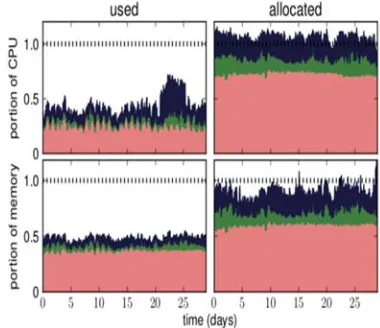
The two types of information about the usage of the resource of jobs running on the cluster included in the trace are the resource requests that accompany each task and the actual resource usage of running tasks. If the scheduler can predict the actual task resource usage and make this prediction more accurate than actual task resource usage that is proposed by the requests, then the tasks could be gathered tightly without loss of performance capabilities. Thus, in [25], the authors determined the actual usage of jobs in a cluster. Although large numbers of tasks are run, the overall usage of the resource should be stable. This stability helps in providing a prediction with better resource usage than resource requests. Figure 3 shows the utilization of the cluster for over 29 days. Utilization is evaluated according to the resource consumption measured (Figure’s left side) and “allocations” (Figure’s right side represents the resources requested from running tasks) [16]. Based on task allocations, the cluster is booked heavily.
Resources total allocation at nearly all times accounts for greater than 80% of the capacity of the memory of cluster and greater than 100% of the CPU capacity of the cluster. However, overall usage is low: averaging over one h windows, the usage of memory does not override approximately 50% of the cluster’s capacity, and the usage of CPU does not override approximately 60% [16].
2083 memory of kernel-managed that required. We use the measurements of utilization that represent the CPU average and the utilization of memory over the measurement period [25].
[image:8.612.99.289.256.420.2]In actual utilization of computing, the trace has been separated into 5 min sampling periods. During a period, for each task usage record available, we calculate and use CPU and memory usage average sum results weighted by the measurement’s length. We do not try to recompense for records usage missing [16].
Figure 3: Moving hourly average of CPU (top) and memory (bottom) utilization (left) and resource requests (right). Stacked plot by priority range, highest priorities (production) at the bottom (in red/lightest color), followed by the middle priorities (green), and gratis (blue/darkest color). The dashed line near the top of each plot shows the total capacity of the cluster [16].
The trace providers state that missing records may result from “the monitoring system or cluster [getting] overloaded” and from filtering out records “mislabeled due to a bug in the monitoring system” [4].
In the following sections, we aim to cover our research steps which are divided into two main steps, the first step is data download and processing technique, the procedures, and codes which been used to accomplish this process. The second step, is data analysis, codes, algorithms, databases, procedures, and techniques that used to analyze the big bulk of data to find the result that we will depend on in our research aims, conclusions, and future works.
7. DOWNLOAD TECHNIQUE AND PROCESS
The cluster data-2011-2 trace data recording starts at 19:00 EDT on Sunday, May 1, 2011 [26]. The time zone of the data center is US Eastern. These settings coincide with the trace timestamp of 600 s. All details of the trace described in the supporting documentation within the package called schema document [4]. This package contains all of the features of the tables, columns, data types, and data maps of all the data of the cluster dataset.
This trace has multiple priorities, which range from 0 to 11 inclusively, with the large number denoting “more important.” Here, 10 is a “monitoring” priority; 9, 10, and 11 are “production” priorities; and 0 and 1 are “free” priorities [25].
An older version of the cluster dataset is called cluster data-2011-1, which represents the first version of this free data. Meanwhile, cluster data-2011-2 trace is identical to the old version, except for a single difference, which is the addition of a single new column of data in the “task_usage” tables. The specific work of this new data is to conduct random picking of 1 s samples of CPU usage from within the linked 5 min usage-reporting period for that task. The use of this trace dataset enables the building of a randomized model of the utilization of the task over time for long-running tasks [26].
The Google cluster trace records the behavior of activities in a single cluster of approximately 12,500 machines [4]. After the download operation is completed, the first step should be processing the trace dataset to decompress it from a single large-sized file into multiple files. These files distributed on numerous folders representing a table of cluster datasets with a single schema (.CSV) file. This file contains the schema details and column data types of all of the contents of the cluster dataset.
2084 These records represent jobs, tasks, processes, or requests of all operations in the cluster. Each job, task, and request have unique IDs for identification and linking to other table contents.
The trace stored in Google Storage for Developers in the bucket called cluster data-2011-2. The total size of the compressed trace is approximately 41 GB. We should access Google storage, which is a service to provide file storage solutions owned and available from Google cloud, to download the trace dataset. Google Storage is not identical but quite similar to Amazon S3 because it provides many useful functionalities, such as bucket synchronization, signed URLs, parallel uploads, and collaboration bucket settings; it is also S3 compatible. “gsutil,” the associated command line tool, is part of the “gcloud” command line interface [27].
“gsutil” is a Python application that provides the capability to access the cloud storage using its command line. “gsutil” can be used to submit various ranges of object and bucket management functionalities, including the following [27].
• Bucket creating and deleting
• Object downloading, uploading and deleting • Object and bucket listing
• Object copying, renaming and moving • Bucket and object ACL editing
We need to access Google cloud SDK through a developer account to obtain the authority to download the cluster dataset bucket, as well as a cluster dataset using the Google cloud SDK “gsutil” command line tool. “gsutil” uses the “gsutil cp” code, which is a copy command to copy the cluster dataset file from Google cloud into a PC.
gsutil cp -R dir gs:// clusterdata-2011-2 “path in PC” The download operation starts to copy all the bucket data clustered dataset files from cloud storage into a PC. Here we would like to highlight one of this paper’s main contributions which are the amount of downloaded data, which considered as unusual amount for considerable number of researchers who worked on google cluster trace dataset, that is, when we did our research, we found that almost all researchers could download only (25,000,000)
records of data. To exceed this amount of data, we would use our google developer account to access Google Cloud SDK and using "gsutil" python application to gain the accessibility to all available data of google cluster trace dataset which we have it now as an offline data for researched prepuces. The offline data which we have now represents all of cluster data-2011-2 data which exceeds 1,500,000,000 records of data stored into (.CSV) data files compressed as (.gz) files distributed over multiple folders each one represents a data table of cluster trace dataset with a schema file to describe its distribution and data types.
We need to process the compressed data by decompressing and integrating them with one of the database servers. In this study, we use the SQL Server 2012 Enterprise Core Edition. We use the (C#) programming language code for the operation to decompress the (500 (.gz) file) pragmatically. Chart 1, demonstrations the workflow of decompression programming code.
The result of the decompressing operation is a folder called the cluster dataset table. Each folder contains a (500 (.gz) file), which is a compressed file containing a single (.CSV) data file.
2085
Chart 1: Decompressing the programming code steps.
The next step is to import all 500 (.CSV) data files into the SQL server database to gather multiple sets of separated data into one table in single database places inaccessible SQL Server to process and analyze them as a single data table. We use the C# code to import the files automatically into the data server in a sequential methodology to keep the original data ordering.
In the next section, we are implementing an analysis using SQL programming language in order to perform K-means algorithm on uploaded data collected into a single data table located in SQL Server enterprise edition (2012) database in order to find a cluster of data.
Chart 2, demonstrations the workflow of files import into SQL server programming code.
Chart 2: Importing the CSV files into the SQL server pragmatically using the code steps.
8. DATA ANALYSIS USING SQL SERVER
To enhance the performance of the cloud environment, we aim to analyze the large number of data selected from Task_Uage table to be clustered as some groups depending on their CPU_rate. We will use the K-means clustering algorithm for clustering operation, and it will execute on SQL server environment using SQL programming language.
Define FileStream Object
FileInfo fileToDecompress
Extract GZipStream from each GZ compressed file
CompressionMode.Deco mpress
write an excracted CSV file
decompressionStream.Copy To
Get the files to be Decompressed
fileToDecompress.FullN ame
Read the name of each file
fileToDecompress.Open Read()
Declare Variable and set values
define CSV files path
select file path
provide the file delimiter
if file empty Define DB server path Log in to the
server
Open server connection
Select DB from server
select table to insert data in
No Yes
Next File
Prepare insert
2086
8.1.SQL Server
Microsoft released the SQL Server for OS/2, which began as a port Sybase SQL Server onto OS/2 in 1989 as a project of Sybase, Ashton-Tate, and Microsoft [28].
This project has been through many stages of development until the last release (SQL Server 2017). The developed version of the SQL Server represents a relational database management system. As a database server, this software product provides the primary function capability of storing and retrieving data as requested by other software applications, which may run on a local host computer or over network-linked computers (including the Internet). A dozen different editions of Microsoft SQL Server have been made by Microsoft [29]. Each version provides different support for different audiences and for a range of workloads, which could cover either large Internet-facing applications with many concurrent users or single small machines. Multiple editions of Microsoft SQL Server have been made by Microsoft, with different feature sets to cover different user’s requirements. These editions are presented and utilized in [28, 29] such as Enterprise Edition which managed databases of up to 524 petabytes and could address 12 terabytes of memory size with the capability of supporting of 640 logical processors (CPU cores).
In [30] Standard Edition which comes in two phases of services, namely, core database engine and stand-alone services, Web Edition which described as a low-TCO option for web hosting. While in [28], Business Intelligence which supports capabilities and tools include the Standard Edition and Business Intelligence tools: Power View, PowerPivot, BI Semantic Model, Data Quality Services, Master Data Services, and xVelocity in-memory analytics.[31], Workgroup Edition which provides the functionality of a core database but does not provide additional services [32], and finally the Express Edition which is a scaled down, free edition, contains a core database engine.
8.1.1. Overview
In this section, we will start with data analysis by using the K-means clustering algorithm. We will analyze (50000000) record of (Task Usage Table), which is the updated table of clusterdata-2011-1, in which clusterdata-2011-2 trace is identical to the old version except the addition of a new column of data in the “task_usage” tables [26], in addition to column
update that we mentioned above. The data of the table contains many columns which could
represent the primary information that could be used to gain data analysis, the analysis will work on Task Usage Table in order to classify the tasks in the table according to its CPU rate consumption, to do this we need to build clustering module to use CPU_rate as an attribute.
Using K-means clustering algorithm, we will Cluster data of (50,000,000) record of Task Usage Table, using an operational environment with the specifications below:
• Win 10 operating system. • 8 GB RAM.
• CPU Core-i-5. • Hard 1 TB (HD).
• SQL Server enterprise edition (2012). • SQL Management Studio (2012).
8.1.2. K-means clustering algorithm
The definition of clustering could be described as the combination of a number of objects in a single group which are comparable between them and non- comparable to another sets. It is extensively mining, image processing, image processing and analysis, web cluster engine, analysis of weather report, bioinformatics, etc. [33]. Several methodologies of the clustering had been used such as density-based, model-based, grid-based method, hierarchical, etc. K-means [34] clustering algorithm is an unsupervised learning algorithm which used with unlabeled data, i.e., data not classified into any groups or cluster. The objective of this algorithm is to find the clusters in the data with the already given number of clusters. The number of clusters and the dataset is the inputs of the algorithm. The dataset is the collection of data for each data point. The number of groups can either be randomly selected or randomly generated from the dataset. The algorithm works as follows: firstly, initialize the number of clusters and the set the centroid of the groups. Each data point assigned to a cluster based on the smallest distance between the centroid and the data point. The centroids are updated or recomputed by taking the average (mean) of the data point assigned to the cluster. The process continues until the stopping criterion met. The stopping criterion is any one of them which are data points is not changing the groups, the sum of distances minimized or the number of iterations reached the maximum.
8.1.3. Process and results
2087 average of CPU_rate value had been calculated. Class assigning over attributes step is the second step of the process which performed in order to choose a random class point from attribute data, this operation output saved as a data table with (25,344) class values record Figure 4.
Figure 4: Random selected centroid distributed over three classes.
Each value represents a random "Centroid," in which each centroid is used by the next step of clustering operation as Mean (K). The classifier that been resulted is used to analyze the data by classifying it and thereby produce initial clusters abound an initial set of centroids randomly, each centroid after that arithmetically sets to the cluster's mean that defines. The centroid selecting and allocation process which leads to adjustment of the centroid is keep repeated in order to re-adjust centroid until the centroid's values are stabilize.
The result of 50,000,000 record clustering using SQL programing language over SQL Server Enterprise Edition (2012) is described using a simple data table which explains the effects of clustering. The data groups into three clusters each of which has its own (freq.) which represent the number of records in each cluster and (avg_CPU_rate) which represents the Average of CPU Rate in each cluster that will be the most effective factor in future task distribution over the cluster machines. Also, the process iteration on all clustering operation during data analysis.
Our analysis process has passed multiple processing steps as in order do the final step which is performing K-means Clustering algorithm as below:
- Data Selecting: Select 50,000,000 record from the overall dataset which is approximately 375,000,000 record.
- Data Cleaning: Remove outliers’ values and null values to start mathematical operations.
- Attributes Calculation: Calculate attribute value for each data values by calculating the:
Attribute value CPU_Rate – Avr CPU_Rate stdev CPU_Rate
For all selected data which is (50,000,000) record. - Random Centroids Selection: Perform a pre-programmed function which we pre-programmed and stored into SQL server to select the number of the random point from the selected data as centroids, each point labeled by a random cluster label from (0-2) due to the number of the cluster we worked on which (3).
- Data Clustering: Use initial value on clusters centroid point and start clustering selected 50,000,000 records then select the next centroid and re-clustering for remaining of 50,000,000 records and repeat this operation until there is no value remaining not linked off the group with one of data clusters.
- Result Saving: Save the resulted data each as a record with its cluster label in the output results table of data that should contain 50,000,000 records of the cluster and labeled data. Each record also contains the Job ID of the original data in order to study the other fields of each record and do the experiments and set the relations to other data such as (Memory Rate, Time Stamp, and so on), that could be more efficient in performance enhancement in the cloud. Each Job record in the data table (Task Usage Table) related to a machine in the cloud environment by “Machine ID” field, this relationship will be used to identify the machines which should be in each cluster based on the job record in that cluster. Depending on this clustering allocation for cloud machines, future job will be allocated to the most suitable cluster of machined which provide its CPU usage need.
The result could be described as below: No Clusters: 3.
Data AVR over the clusters:
Table 3: Statistical Results of K-meansdata
clustering.
0 5000 10000 15000 20000 25000
Total 24675
604 65
0
1
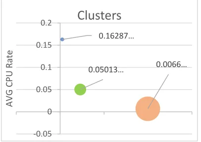
2088 cluster freq avg_CPU_rate
0 39888524 0.00669755514227397 1 9149318 0.0501349851423366
2 962158 0.162876877451737
The elapsed time of clustering operation: 31 hours, 17 minutes, and 32 seconds. Process iteration: 288.
[image:13.612.277.526.48.239.2]As shown in Figure 5 each cluster has a CPU rate average; this average could use to predict the cluster of upcoming tasks over cloud which require CPU usage to minimize the time of tasks distribution over all cluster nodes. In this case, the cloud gained the ability to allocate the upcoming task to the most suitable group of nodes or to the most suitable node depending on the CPU rate which requested by the upcoming task.
Figure 5: the average of CPU rate in Each Cluster.
In Figure 6, we note that the three clusters distributed over the dataset, the size on each cluster depends on the number of tasks (Points) which allocated within the cluster. When we made a comparison between the cluster in Figure 4 and Figure 5, we found that the most significant cluster is in the cluster which has the minimum average of CPU rate even it has the most significant number of tasks (Points) allocated together.
Figure 6: Clusters distribution over the data set.
Data processing that performed in this paper conducted to create three groups of data represents a cluster of tasks which been served by the cloud cluster machines, distributed according to each task CPU rate requirement. Each cluster has its CPU average which considered as a primary factor of future tasks allocation in the cloud cluster. According to these clusters, the upcoming tasks which need to be served by the cloud cluster machines will be oriented to the most suitable group of machines that have available CPU power equal or near to the CPU rate that needed by that upcoming task. This allocation solution will help in decrease the time wasted in common scheduling techniques and also decreases the storage and network bandwidth that wasted by the upcoming task which takes a long time to find an optimal selection of machine to be performed on or waiting the current running machines to be free. Thus, this technique could be considered as pre solutions which provide a guide for task allocation based on pre performed task resource usage compared and linked with the resource capacity and availability of cloud cluster machines in order to enhance the cloud environment's performance.
9. CONCLUSIONS AND FUTURE WORK
The Analysis of Google trace data which we demonstrate in this paper targets a large number of task usage data which represents all the requirements of each task that operates in google cloud during the period of google cluster dataset recording. These data records, play a significant role in cloud environment performance regarding its importance to identify each task’s usage requirements. By analyzing (50,000,000) records of task usage data, we produced some clusters containing a significant 0.0066…
0.05013… 0.16287…
‐0.05 0 0.05 0.1 0.15 0.2
AVG
CPU
Rate
Clusters
No. Points 39888524
No. Points 9149318
No. Points 962158
‐10000000 0 10000000 20000000 30000000 40000000 50000000
No.
Points
[image:13.612.94.297.336.480.2]2089 number of tasks, each of which had been run on a single machine in the cloud cluster and linked to that machine by “Machine ID” field in the task data Depending on this relationship, we could select the machines of each produced cluster to calculate the availability of CPU usage of each. This calculation will be the millstone of future tasks allocation over cloud cluster machines depending on its resources availability and its suitability to future task resource requirements.
As a conclusion of this paper, we conclude that the tasks allocation and distribution over suitable resources available clusters of machines have a significant impact in performance enhancement especially when the number of clusters is substantial and the data of clustering operation was randomly selected.
Depending on the results of a significant number of task resources and usage data analysis, the cloud machine resources availability, and workload could be predicted precisely. By this prediction and based on the resource availability of each group of machines in the cloud cluster in addition to the task requested resources, the new and upcoming task could be oriented and allocated to the most suitable group of machines or specific machine. In which provide almost full needed resources and process efficiency which is better than any other machine in the cloud cluster. This analyses and pre-allocation of tasks on the cloud cluster considered as an initial solution to reduce task scheduling waiting for time plus storage and network bandwidth loss. Our study provides a reliable solution to enhance the performance of the cloud environment to be one of the proposed solutions by cloud computing field researchers.
As a future work, we aim to analyze the more massive amount of data to find a new group (Cluster) within its point. By doing that, we strive to facilitate the work of tasks distributions over Cloud cluster nodes to enhance the cloud environment’s performance. Also, we aim to use Hadoop Ecosystems for dumping the cluster analysis big data and use more predictive analysis algorithm with the tools available in Hadoop systems. To get better enhancement of distribution of trace analysis data and represent these results by CloudSim in order to simulate the cloud tasks process and allocation and determine the enhancement of could environment performance.
REFERENCES
[1] M. Alam, K. A. Shakil, and S. Sethi, "Analysis and clustering of workload in google cluster trace based on resource usage," in Computational Science and Engineering (CSE) and IEEE Intl Conference on Embedded and Ubiquitous Computing (EUC) and 15th Intl Symposium on Distributed Computing and Applications for Business Engineering
(DCABES), 2016 IEEE Intl Conference on,
2016, pp. 740-747: IEEE.
[2] C. Pelletingeas, "Performance evaluation of virtualization with cloud computing," Edinburgh Napier University, 2010. [3] M. Alam and K. A. Shakil, "Cloud database
management system architecture," UACEE International Journal of Computer Science
and its Applications, vol. 3, no. 1, pp.
27-31, 2013.
[4] C. Reiss, J. Wilkes, and J. L. Hellerstein, "Google cluster-usage traces: format+ schema," Google Inc., White Paper, pp.
1-14, 2011.
[5] Y. Chen, A. S. Ganapathi, R. Griffith, and R. H. Katz, "Analysis and lessons from a publicly available google cluster trace,"
EECS Department, University of California, Berkeley, Tech. Rep.
UCB/EECS-2010-95, vol. 94, 2010.
[6] A. Al-Dulaimy, W. Itani, R. Zantout, and A. Zekri, "Type-Aware Virtual Machine Management for Energy Efficient Cloud Data Centers," Sustainable Computing:
Informatics and Systems, 2018.
[7] A. Aldulaimy, R. Zantout, A. Zekri, and W. Itani, "Job classification in cloud computing: the classification effects on energy efficiency," in Utility and Cloud Computing (UCC), 2015 IEEE/ACM 8th
International Conference on, 2015, pp.
547-552: IEEE.
[8] A. Al-Dulaimy, A. Zekri, W. Itani, and R. Zantout, "Paving the Way for Energy Efficient Cloud Data Centers: A Type-Aware Virtual Machine Placement Strategy," in 2017 IEEE International
Conference on Cloud Engineering (IC2E),
2017, pp. 5-8: IEEE.
[9] J. Wilkes, "More Google cluster data,"
Google research blog, Nov, 2011.
2090
International Wireless Communications &
Mobile Computing Conference (IWCMC),
2018, pp. 1167-1172: IEEE.
[11] Z. Liu and S. Cho, "Characterizing machines and workloads on a Google cluster," in Parallel Processing Workshops (ICPPW), 2012 41st International
Conference on, 2012, pp. 397-403: IEEE.
[12] O. Beaumont, L. Eyraud-Dubois, and J.-A. Lorenzo-del-Castillo, "Analyzing real cluster data for formulating allocation algorithms in cloud platforms," Parallel
Computing, vol. 54, pp. 83-96, 2016.
[13] S. Yousif and A. Al-Dulaimy, "Clustering cloud workload traces to improve the performance of cloud data centers," in
Proceedings of the World Congress on
Engineering 2017,(WCE2017), 2017.
[14] S. Di, D. Kondo, and W. Cirne, "Characterization and Comparison of Google Cloud Load versus Grids," 2012. [15] F. Gbaguidi, S. Boumerdassi, E. Renault,
and E. Ezin, "Characterizing servers workload in cloud datacenters," in Future Internet of Things and Cloud (FiCloud),
2015 3rd International Conference on,
2015, pp. 657-661: IEEE.
[16] C. Reiss, A. Tumanov, G. R. Ganger, R. H. Katz, and M. A. Kozuch, "Heterogeneity and dynamicity of clouds at scale: Google trace analysis," in Proceedings of the Third
ACM Symposium on Cloud Computing,
2012, p. 7: ACM.
[17] M. Alam and K. A. Shakil, "A decision matrix and monitoring based framework for infrastructure performance enhancement in a cloud based environment," arXiv preprint
arXiv:1412.8029, 2014.
[18] M. Alam and K. A. Shakil, "An NBDMMM Algorithm Based Framework for Allocation of Resources in Cloud," arXiv
preprint arXiv:1412.8028, 2014.
[19] D. Zhang, P. Coddington, and A. L. Wendelborn, "Improving data transfer performance of web service workflows in the cloud environment," International Journal of Computational Science and
Engineering, vol. 8, no. 3, pp. 198-209,
2013.
[20] W. Huang, J. Liu, B. Abali, and D. K. Panda, "A case for high performance computing with virtual machines," in
Proceedings of the 20th annual
international conference on
Supercomputing, 2006, pp. 125-134: ACM.
[21] A. K. Mishra, J. L. Hellerstein, W. Cirne, and C. R. Das, "Towards characterizing cloud backend workloads: insights from Google compute clusters," ACM SIGMETRICS Performance Evaluation
Review, vol. 37, no. 4, pp. 34-41, 2010.
[22] Q. Zhang, M. F. Zhani, S. Zhang, Q. Zhu, R. Boutaba, and J. L. Hellerstein, "Dynamic energy-aware capacity provisioning for cloud computing environments," in
Proceedings of the 9th international
conference on Autonomic computing, 2012,
pp. 145-154: ACM.
[23] Q. Zhang, J. L. Hellerstein, and R. Boutaba, "Characterizing task usage shapes in Google’s compute clusters," in
Proceedings of the 5th international workshop on large scale distributed
systems and middleware, 2011, pp. 1-6: sn.
[24] A. Tumanov, J. Cipar, G. R. Ganger, and M. A. Kozuch, "alsched: Algebraic scheduling of mixed workloads in heterogeneous clouds," in Proceedings of the third ACM Symposium on Cloud
Computing, 2012, p. 25: ACM.
[25] C. Reiss, A. Tumanov, G. R. Ganger, R. H. Katz, and M. A. Kozuch, "Towards understanding heterogeneous clouds at scale: Google trace analysis," Intel Science and Technology Center for Cloud
Computing, Tech. Rep, vol. 84, 2012.
[26] Google. (2011). Google cluster data blob
master on github.com. Available:
https://github.com/google/cluster-data/blob/master/ClusterData2011_2.md [27] A. P.-D. Science. (2018). Top gsutil
command lines to get started on google
cloud storage. Available:
https://alexisperrier.com/gcp/2018/01/01/g oogle-storage-gsutil.html
[28] Wikipedia. (2018). Microsoft sql server.
Available:
https://en.wikipedia.org/wiki/Microsoft_S QL_Server
[29] M. Corporation. (2007). Sql server
compare editions. Available:
http://www.microsoft.com/sqlserver/en/us/ product-info/compare.aspx
[30] M. Corporation. (2011). Sql server 2008
editions. Available:
2091 [31] M. Corporation. (2013). Database system |
performance & scalability | sql server 2012
business intelligence editions. Available:
http://www.microsoft.com/sqlserver/en/us/
editions/2012-editions/business-intelligence.aspx
[32] M. Corporation, "Sql server 2012 licensing datasheet," 2011, Available: http://download.microsoft.com/download/
a/5/d/a5d112e1-78ff-491f-9364-f1bc6fae7d57/sql_server_2012_licensing_ datasheet_nov2011.pdf.
[33] L. Bijuraj, "Clustering and its Applications," in Proceedings of National Conference on New Horizons in
IT-NCNHIT, 2013, p. 169.
[34] J. MacQueen, "Some methods for classification and analysis of multivariate observations," in Proceedings of the fifth Berkeley symposium on mathematical
statistics and probability, 1967, vol. 1, no.
![Table 1: Machines percentage of each memory capacity level [1].](https://thumb-us.123doks.com/thumbv2/123dok_us/8899943.954487/6.612.98.290.194.507/table-machines-percentage-memory-capacity-level.webp)