Who benefits from Child Benefit?
Laura Blow, Ian Walker and Yu Zhu
No 749
WARWICK ECONOMIC RESEARCH PAPERS
Who benefits from Child Benefit?
Laura Blow*, Ian Walker**, and Yu Zhu***
* Institute for Fiscal Studies, 7 Ridgmount Street, London WC1E 7AE, UK ** Department of Economics, University of Warwick, Coventry CV4 7AL, UK *** Department of Economics, University of Kent, Canterbury CT2 7NP, UK
Version 3.1
Thursday, 09 February 2006
JEL codes: I38, D79, D12
Keywords: altruism, child poverty, intra-household transfers
Abstract
Over much of the developed world governments make significant financial transfers to parents with dependent children. For example, in the US the recently introduced Child Tax Credit (CTC), which goes to almost all children,
costs almost $1billion each week, or about 0.4% of GNP. The UK has even
more generous transfers and spends about $25 a week on each of about 8 million children – about 1% of GNP. The typical rationale given for these transfers is that they are good for our children and here we investigate the effect on household spending patterns. The UK is an excellent laboratory to address this issue because such transfers, known as Child Benefit (CB), were simple lump sum universal payments for a period of more than 20 years. We do indeed find that CB is spent differently from other income – paradoxically, it
appears to be spent disproportionately on adult-assignable goods. In fact we
estimate that more than half of a marginal pound of CB is spent on alcohol. We resolve the puzzle by showing that the effect is confined to unanticipated variation in CB so we infer that parents are sufficiently altruistic towards their children that they completely insure them against shocks.
* This research was funded by Her Majesty’s Treasury’s Evidence Based Policy Fund with the support of the Department for Education and Skills, Department of Work and Pensions, Department of Culture, Media and Sports, and the Inland Revenue. Material from the Family Expenditure Survey is Crown Copyright and has been made available by the Office of National Statistics through the Economic and Social Research Council’s Data Archive at the University of Essex. The data is used with the permission of Her Majesty’s Stationery Office. We are grateful for comments from Mike Brewer at the Institute for Fiscal Studies, Mike Bielby, Ilona Blue and Mario Pisani of the Inland Revenue, Andrew Oswald at Warwick, and seminar participants at the Department for Education and Skills, the Department of Work and Pensions, the University of Warwick, the University of Kent, the Cardiff Business School, and Queen Mary and Westfield College of the University of London. Needless to say, the opinions are those of the authors alone.
1. Introduction
Over most of the developed world huge financial transfers are made to parents by virtue of their parenthood. For example, in the US the recently introduced Child Tax Credit (CTC), which goes to the vast majority all children1, costs almost $1
billion each week, or about 0.4% of GNP. The UK government spends in total about $25 (at present exchange rates) each week on each child in the form of a lump sum transfer called Child Benefit (CB) which goes to all children, and in addition the UK has its own version of CTC which goes to almost all families with children – and together CB and CTC account for approximately 1% of GNP2.
The typical rationale for these payments that are ostensibly earmarked for children is that they are good for our children. Such transfers are usually motivated by concern for the welfare of children and implicitly presume that there is some market failure that prevents parents from investing in the desired quality and/or quantity of children throughout their lives. This might arise, for example, through child quality being a household public good implying parental free-riding in quality investments, or through imperfections in fertility control. Moreover, particular concern arises for children in poor households, and the US and the UK are distinctive in having child poverty rates that are considerably higher than that in most other countries3. Thus, there may be credit market constraints that prevent households, especially poor ones, from spreading the costs associated with children across their lifetimes.
This paper is concerned with the impact of exogenous changes in a lump sum cash transfer that is made to all parents on their household spending patterns. The UK is an excellent laboratory to address this issue because CB were simple lump sum universal transfers for a period of more than 20 years, prior to the introduction to CTC which was means-tested. Moreover, the level of payments has varied dramatically over time. To anticipate our findings we show that CB is spent differently from other sources of income – but, by and large, it is spent, at the margin, on adult-assignable goods. Indeed, our benchmark results for couples with one child suggest that more than half of a marginal unit of CB is spent on alcohol.
1 See Burman and Wheaton (2005).
2 See Bradshaw and Finch (2002) for details of 22 countries.
Dickens and Ellwood (2003) show that (relative) child poverty (after deducting housing costs) in the UK has grown considerably over time4 from around
15% in 1978 to around 32% in the early to mid 1990’s and that it has fallen only slightly since then to approximately 30% in 2000/15. They go on to show that, although the US has conventionally used an absolute measure and this has fallen consistently since the early 1980’s, a relative poverty measure comparable to the one used in the UK has remained at around 35% since the early 1980’s6. Since much of the policy concern over child poverty arises because of the possible sensitivity of child development to parental resources these figures are alarming. The existence of this sensitivity is supported by the strong correlation between low parental income and bad child outcomes. Many outcome dimensions have been considered in the literature. In the UK, for example, Gregg, Harkness and Machin (1999) find that poor long term health, involvement in crime, low wages, and low levels of educational achievement are associated with earlier low parental incomes. Similar findings have been reported in the US (see, for example, Currie (1994) and Mayer (1997)) and a review of the evidence, including the extent to which such correlations are causal, can be found in Haveman and Wolfe (1995). Indeed, in many countries governments make financial transfers to children via one or both of their parents: all EU countries make such transfers, as do most OECD countries. In some countries such transfers are contingent on household income, while they are lump-sum in others7. The USA recently introduced, and subsequently extended, a Child Tax Credit that also makes such transfers which are now worth $1000 per child per year across almost the whole of the income distribution. In the UK the Child Benefit (CB) programme provides a transfer, usually made monthly and almost invariably to mothers, which is equivalent
4 See also Gregg, Harkness and Machin (1999) who use UK data from the Family Expenditure Surveys
from 1968 to 1996 to show that the proportion of dependent children who live in households with incomes below 60% of median income (the official UK definition of child poverty) had grown from 10% in 1968 to 35% in 1996.
5 See Brewer, Clark and Goodman (2003) for an explanation of recent UK changes in child poverty.
6 However, the National Centre for Child Poverty constructed a relative measure of US child poverty
(defined as having a household income below double the Federal poverty level) and found that this rose from 16.2% of children in 1979 to 22.5% in 1993 and then fell back to 18.7% in 1998 (see Bennett and Hsien-Hen (2000)).
7 In addition many in-kind transfers are made either to parents or directly to the children, such as free or
to approximately 5% of average household total expenditure – and considerably more for poorer households8.
To the extent that the association between child poverty and poor child outcomes is a causal effect, this evidence provides some motivation for child poverty policy. Indeed, the UK government has recently adopted an explicit long run objective of eliminating child poverty. Although CB is universal (i.e. not means tested) it clearly contributes to a reduction in child poverty9. In any event, it seems plausible that lessons that we learn here from this universal programme applies to means tested transfers that are explicitly aimed at relieving child poverty10. CB, in 2003, was worth £16.05 ($28) per week for the first child11, and £10.75 ($19) for subsequent ones, and this has recently been joined by the Children’s Tax Credit which is a further programme that provides a tax credit for children worth £10.40 ($18) per household per week structured in such a way that its value only falls as income rises at a level of income that is far above the mean level of household income12. This credit was further superseded in April 2003 by the Child Tax Credit (CTC), worth slightly more than the Children’s Tax Credit and where the means testing starts higher up the income distribution. The total of all child-related cash benefits amounts to 2% of GDP in 2003 in the UK, compared to 1.5% in the late 1970’s, despite the dramatic fall in fertility. Indeed, the recent reforms to the welfare system have been driven by the desire to
8 For couples (lone mothers) with 1, 2 and 3 children CB as a percentage of total expenditure are 3.8
(10.4), 6.6 (14.8), and 9.1(17.1) respectively. In addition to CB there are supplements to other welfare programmes that depend on the children in the household. The UK relies largely on cash support but also has some in-kind transfers (nutrition supplementation, support for housing costs, and vouchers and hypothecated transfers for childcare which are all means-tested, as well as the medical cover provided to all under the National Health Service).
9 In a speech at the 1999 SureStart Conference, the Chancellor Gordon Brown described child poverty
as “a scar on the soul of Britain” and said that increases in Child Benefit under the Labour government were part of “immediate and direct action” to provide “cash help to lift children out of poverty”.
10 Income Support (IS) and Job Seekers’ Allowance (JSA), the out-of-work welfare programmes
(mainly for poor lone parents, the disabled and the unemployed), have also benefited from increasingly generous additions for dependent children, as has Working Families’ Tax Credit (WFTC), the main in-work welfare programme.
11 £17.55 per week for a lone parent who has been entitled to the supplementary One Parent Benefit
(OPB) since prior to April 1998.
12 WFTC and Children’s Tax Credit has recently been replaced by Working Tax Credit (WTC) and
ensure that absolute cash support for children is independent of parental circumstances such as unemployment, sickness and disability13.
Our aim here is to try to complement existing research on the relationship between child outcomes and household income by trying to infer how CB is spent – in particular, we are interested in how CB affects spending on adult and child specific goods. That is, we investigate the impact of Child Benefit on household spending patterns with a view to estimating its impact on goods that are “assignable” to either children or adults. Thus, this paper takes a direct approach as to whether “money matters” by investigating the effect of variations in transfers to households with children on household spending decisions. We seek to establish the extent to which they affect household spending decisions since this is one mechanism through which a causal effect may operate. We are particularly concerned with spending on “child goods” and use spending on children’s clothing to reflect this. In contrast, we also look at how transfers to parents affect spending on “adult goods” and use alcohol, tobacco, and adult clothing as examples of these14.
Our headline finding is that CB is spent differently from regular income – but it is spent disproportionately on adult-assignable goods. We resolve this paradoxical finding when we disaggregate our variation in CB into anticipated (inflation-driven) variation and unanticipated (reform-driven) variation. Our conclusion is that it is only the unanticipated variation in CB, driven by policy changes, that is allocated differently to regular sources of income. Thus, it is parents who benefit from unanticipated variation in Child Benefit – a result that is consistent with the view that parents are altruistic towards their children and so insure them against income shocks.
The plan of the paper is as follows: Section 2 outlines the existing literature on child outcomes and parental incomes which motivates our analysis and reviews the few existing papers that investigate spending patterns; section 3 summarises our data on CB variation and on household spending patterns; section 4 provides our empirical findings that relates the two; and section 5 concludes.
13 See Adam and Brewer (2004) for a review of the development of all UK child-related benefits
including CB.
14 Our analysis is one of a complete demand system where we impose the adding up condition. Thus
2. Literature
There is an extensive literature that establishes strong correlations between child outcomes and parental incomes, whereas there is comparatively little evidence to show that giving poor parents more money makes for better children. Indeed, rather few studies attempt to establish the causal effect of parental incomes on child outcomes. The evidence points to child poverty being strongly associated with bad child outcomes but the evidence that reducing financial poverty is good for those outcomes suggests small, and generally insignificant, effects. While the presumption behind child-oriented cash transfer programmes is that children do indeed benefit from them, it turns out that we have little quantitative evidence to support this.
For the USA, Mayer (1997) examines how rich, middle-class, and poor parents spend their income on items that may be helpful to child development. Differences in spending, across income groups, on items regarded as necessities, such as shelter, food consumed at home, and health care, are far narrower than differences in spending on less essential items. The result is that the difference in resources available to poor and middle-class youngsters is typically quite small. Mayer finds that very poor children see doctors almost as frequently, and live in homes that are almost as un-crowded, almost as clean, and only a little less likely to have air conditioning or central heating, as middle-class children. Mayer argues that these differences are small because low-income parents devote a large percentage of their income to purchasing items they regard as important for their own or their children's welfare.
alternative strategies to identify the effect of extra family income, she finds that the causal effects of extra income turn out to be modest in magnitude and the conclusion is compelling: income inequality is not an important causal determinant of the unequal opportunities that children face15.
Economists take it for granted that giving additional income to individuals will improve their welfare. But understanding how important giving additional income to parents is likely to be for the well being of their children is more complex. This is because children depend on the behaviours and decisions made by their parents to determine how much, and in what way, they will benefit from additional income into the household. Most straightforwardly, parental income could be important for child outcomes because parents could use additional income to buy goods and services that are good for their children and represent an investment in their children’s future well being. Such theories of parental investment in their children have been the focus of many economists’ thinking about the role of parental income in determining children’s outcomes (see Becker and Tomes (1986)).
Recent work on spending on child and adult clothing by Kooreman (2000) for the Netherlands suggest that the fact that the money is labelled as child benefit motivates households to indeed spend it disproportionately on child goods essentially because of a “mental accounting” effect16. That paper exploits differential variation in CB by age of child for one-child households and finds that the estimated marginal propensity to spend on child clothing is higher for CB than for other income and so argues that this is evidence of a “labelling effect”. However, identification relied on a single change in the rate for young children versus older children that was almost coincident with the change in the payment mechanism. Under this reform the recipient, in the overwhelming number of cases, ceased to be the head of household
15In the same vein, Shea (2000) uses US PSID data, and instruments parental incomes, to show that
“exogenous” variation in parental incomes has only small effects on their children’s abilities. In that paper the estimates exploit the income variation due to union status, industry, and job loss as instrumental variables. Duflo (2000) uses a South African data where black pensioners were given substantial increases in pension incomes in a “natural experiment”. Using a simple difference in differences methodology the author shows that exogenous increases in the incomes of grandmothers makes for better (in terms of nutrition) granddaughters. However, the effect on boys (grandsons) was found to be small, and there was no significant effect of pensions received by men (grandfathers). These latter results suggest that households do not function as unitary entities, so that the effectiveness of public transfer programs may depend on the gender of the recipient.
16 See Thaler (1990) for why this phenomenon might exist and why it leads to differences in marginal
and became the mother17. The only statistically significant finding was for one-child married couples – for larger households and for single mothers there were no significant effects of CB.
Moreover, further work on Slovenia by Edmonds (2002) found no significant effects. However, this work exploited the dependence of Slovenian CB on household income and the number of children in the previous year and so requires that these have no direct effect on current expenditure patterns – something that seems unlikely because of serial correlation in incomes, habit persistence, and the fact that changes in the number of children in the household are likely to be anticipated18.
As in the Netherlands, UK CB over the period 1980 to 2000 was a universal (not means-tested) programme, where payments depended on the current number of dependent children, went to the mother, payments were not subject to taxation, and participation was effectively 100%19. Thus the UK offers an interesting laboratory to study the effect of CB because we do not have to correct for programme non-participation. Indeed it was this absence of selectivity that allowed Lundberg, Pollak and Wales (1997) to investigate the impact of the UK “wallet to the purse” reform in the late 1970’s. The argument for such a reform was that mothers are better agents for their children than fathers. The authors show, in grouped data, that there is an increase in spending on child clothing relative to adult clothing and female adult clothing relative to male adult clothing following the reform which gave mothers control over this source of income. This finding has subsequently been substantiated by Jennifer Ward-Batts (2000) using household level data20. These findings, that household
17 Thus the paper places some weight on the presumption that this “wallet to purse” transfer had an
equal effect on spending patterns across households with different aged children. Since maternal market labour supply may be affected by the intra-household transfer this seems unlikely.
18 Jacoby (2002) investigates in-kind (food) transfers targeted on children and finds no evidence of a
“flypaper” effect of such transfers increasing the calorific intake of the children. Bingley and Walker (2003) consider the effects of giving food and milk to children on household spending patterns – we find significant effects on household milk spending. Schluter and Wahba (2004) examine the effects on household spending patterns of the Mexican Progressa experiment whereby schooling subsidies were randomly assigned. They show significant effects of the subsidy on child clothing expenditure which they interpret as altruistic behaviour. However, the subsidy is conditional on attending schools and it seems likely that this conditionality affects how the money is spent – for example, attending school may itself have an impact on clothing needs.
19 Private correspondence with DWP confirms that this also applies to the supplement to CB that is
paid to lone parents – One Parent Benefit (OPB).
20 Hotchkiss (2005) has noted that the changes in adult spending patterns observed by Lundberg et al
members fail to pool their resources in making spending decisions, have been echoed in other studies21 and suggest a rejection of the unitary model of household behaviour. Here, we abstract from these considerations by only using data post 1979, by which time the wallet-to-purse reform had been fully implemented22, and using the couples samples separately from the lone parents sample. In the latter there is no intra-household issue, while in the former our estimates are conditional on it23.
3. Data and Identification
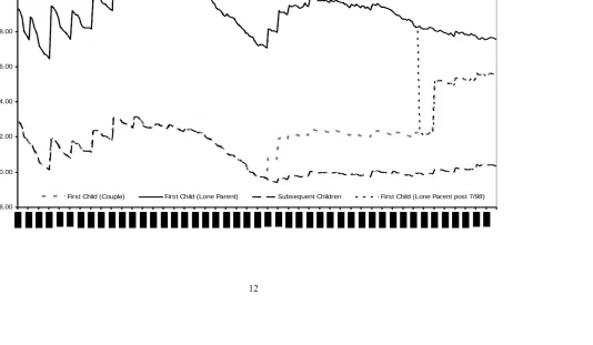
Our analysis covers the 21 years from 1980 (when CB had finally entirely replaced the earlier system of Family Allowances whose main beneficiaries were fathers) to 2000 (after which tax credits for parents were introduced which would complicate our analysis because these credits were means tested and were subject to a potential take-up problem). Across this period there have been wide variations in real CB within years induced by differences in inflation across years, and large changes in the real value of CB between years driven by reforms whereby CB was reflated by more or less than the inflation rate from the previous uprating. For example, a large reform occurred in 1991 whereby CB entitlement of the first child rose by a considerable amount, and a further increase for the first child occurred in 1999. Figure 1 shows the two sources of variation in real CB for first and subsequent children and for lone parents and couples separately24. The sawtooth shape in the 1980’s clearly shows the effects of inflation - something that is not obvious in later years when
21 See Phipps and Burton (1998) and Bourguignon, Browning, Chiappori and Lechène (1993) for
example. However, these studies simply examine whether spending patterns are affected by the individual composition of household income without regard to the potential endogeneity of that composition.
22 Our data record who receives the CB in the household: the proportion of two parent households
where the mother is the recipient is 99.1%.
23 More recently Gregg, Waldfogel and Washbrook (2004) have described how patterns of spending
have changed between 1996/7 and 2000/1, for low income households relative to other households as their relative disposable incomes varied (for a variety of reasons, not just CB). They find that that spending on alcohol and tobacco for low income households with children relative to those with higher income has fallen, and spending on toys, games and clothing and footwear has risen. However, their analysis takes no account of changing composition of the low income group relative to the rest – which will have been dramatic because of the large change in in-work welfare entitlements that occurred in 1999, the introduction of the National Minimum Wage in 1999 and, the unfolding New Deals, especially for lone parents, all of which will have contributed to a reduction in worklessness amongst this low income group of parents. Moreover, there will have been cyclical effects that have more pronounced effects on the bottom of the distribution than the rest.
24 See Greener and Cracknell (1998) for the historical background and development of Child Benefit in
inflation was considerably lower. The real reductions over the period 1984 to 1990 shows the effect of not uprating in line with price inflation in the period when the Conservative government of the day had (implicitly) adopted a policy of targeting support on the very poorest households through real rises in the generosity of the in-work welfare programme for parents (then called Family Credit) at the expense of CB. In 1991 a large real rise in CB for the first child of a couple was introduced – this distinction between first and subsequent children had always been a feature of CB for lone parents (lone parents received a supplement to CB known as One Parent Benefit (OPB) that created this wedge between first and subsequent children) but not for couples. In a controversial change in 1997 the new Labour government abolished the OPB and so effectively eliminated this distinction between couples and lone parents25. However, the adverse effect on (new) lone parents was soon ameliorated when the rate for all first children was subject to a large real increase.
Until 1999, and the Labour government’s commitment to abolish child poverty, the real value of CB was lower than it had been when it was first introduced back in 1978 and that remained the case for the first children of lone parents and for all subsequent children in 2001, and still remains to the present. The real value of CB for the first children of lone parents had fallen by more than 10% while the value for all subsequent children had fallen by more than 15%. It is only with the recent introduction of the supplement to CB known as Child Tax Credit (CTC) that the real values of child-contingent financial support enjoyed by parents back in 1979 have been matched. Our analysis relies on the real variation in CB for given household types. That is, we make no attempt to exploit the variation in CB across household types at a point in time. We do this because we do not want to rely on functional form assumptions that restrict how different numbers of children affect household spending. Moreover, we do not want to make any assumptions about the nature of intra-household distribution of income so we present estimates separately for lone parent households and couples (which include repartnered divorcees). Finally, we also decompose our data into those on in-work welfare (WFTC) and out-of-work welfare (Income Support) and those not. CB interacts with the latter because CB counts as income for the purposes of computing IS payments and nominal CB rises are effectively taxed at 100% - although the situation is complicated by the fact that the
child-related component of IS are also increased over time. We choose not to attempt to exploit this source of variation on the grounds that it may be too subtle for consumers to detect and the group affected is, in any case, quite small. Thus, most of our analysis will be conducted over households who are not on either in-work or out-of-work welfare.
Effectively identification comes from two sources: the variation in inflation rates across years that ensures that we can identify anticipated effects independently of seasonality (effectively we assume that the seasonality in the data is orthogonal to inflation); and from the various reforms that ensure that there are discontinuities in anticipated CB (that cannot account for smooth changes in expenditure patterns).
We use Family Expenditure Survey (FES) data on household spending patterns, which contain detailed household26 expenditure information, constructed from two consecutive weekly diary records supplemented with information about regular payments. The expenditure data is regarded as being quite accurate with the exception of alcohol and tobacco27, which are under-recorded relative to other sources of information. Moreover, there is considerable consistency over time. The data also records sources of income and their levels and periodicity, and the detailed characteristics of respondent households including the number and ages of children28. Table 1 shows the breakdown of the data by household type. Table 2 shows some summary statistics for households with exactly one child.
4. Econometric Analysis
In our parametric work we test for differential marginal propensities to consume out of CB compared to other income for different commodity groups. Unlike earlier research, we model the whole of household (non-housing) spending - both child assignable goods as well as those that are adult-assignable and those that are not
26 Spending data at the individual level is not available in the public use files. However, since 199x the
data has separately recorded the expenditure of all children aged 7-15.
27 See Tanner (1998) for an analysis of the reliability of FES expenditure data. The deficiency in the
alcohol and tobacco categories is thought to be largely associated with differential response rates of smokers and drinkers and not because of under-recording by respondents. We find no evidence that under-recording is correlated with the real variation in CB.
28 We drop all households where the youngest child is 16 and over because the FES treats the clothing
assignable at all (food, and all other non-housing expenditure29). Identification relies on the sizeable real variation in CB over time – at least part of which is discontinuous arising from reforms. Since we exploit only time series CB variation we present estimates in the body of the paper based on samples of households that contain only one child. We assume that expenditure on good i by household h is given by
(
,
)
ih i h h h i ih
e
=
f x CB
+
Ζ
β
+
ε
where xh is household h’s other income30 apartfrom CB (defined as total expenditure minus CB), Zh is vector of exogenous
characteristics such as age and age squared of the household head, dummy variables to control for having a child aged 0-4 and 5-10 (relative to 11-15), region to control for regional differences in spending, and a linear trend31 and a vector of month dummies to capture seasonal variations in spending, and
ε
ih captures theunobservable determinants of spending patterns32.
Since each of the expenditure equations contain the same explanatory variables we estimate the system using the usual Seemingly Unrelated Regression method to allow us to test cross equation restrictions. We impose adding-up in the usual manner of omitting one arbitrary equation. We omit all other expenditure apart from the assignable ones (male, female and child clothing, alcohol, and tobacco) and food so just six equations are reported.
In our parametric analysis below, we further assume that f x CBi
(
h, h)
is linearand additively separable. Linearity here is unlikely to be important – we are estimating a local approximation around the mean of total expenditure and the effect of CB is, itself, (relatively) small variation around that mean. The specification
29 This latter is the excluded category. Homogeneity of demands would allow us to recover the
parameters of this excluded category form the parameters estimated assuming that adding-up holds. The estimates are guaranteed to be independent of which commodity forms the excluded category.
30 We use total expenditure (minus CB) as our explanatory variable rather than income. This is to
ensure consistency with an intertemporally separable lifecycle maximising model. See Blundell and Walker (1986). Results using total (net of tax and welfare) income (minus CB) are essentially the same and are available on request.
31 We included a cubic spline in month of survey to capture smooth changes in tastes but were able to
reject this in favour of a simple linear trend.
32 Estimates which include relative prices are available on request. We do not control for relative prices
12 Figure 1 Real CB 1979-2001 (£ per week in 2003 prices)
8.00 10.00 12.00 14.00 16.00 18.00 20.00 22.00
R
e
a
l c
h
il
d be
ne
fi
t
(£
pe
r we
e
k
)
13 Table 1: Summary statistics: Household types (Numbers and proportions)
1 children 2 children 3+ children
Married Lone All Married Lone All Married Lone All Total Not on 8575 744 9319 12967 570 13537 4502 165 4667 27523
welfare 0.87 0.25 0.73 0.88 0.25 0.80 0.76 0.16 0.67 0.75
On Out of 948 1836 2784 1255 1453 2708 1000 783 1783 7275 work welfare 0.10 0.63 0.22 0.09 0.65 0.16 0.17 0.76 0.26 0.20
On In-work 288 340 628 441 216 657 422 81 503 1788
Welfare 0.03 0.12 0.05 0.03 0.10 0.04 0.07 0.08 0.07 0.05
14
Table 2: Summary statistics: Expenditure Patterns for Households with 1 Child Weekly amounts (£) and standard deviations
Couples Lone Parents
Not on welfare
Out of work
welfare
On In-work
welfare
Total welfare Not on
Out of work
welfare
On In-work
welfare
Total
Expenditure (12.49) 7.72 (8.90) 4.51 (8.49) 5.23 (12.13) 7.34 (15.78) 9.16 (8.35) 4.81 (10.47) 6.60 (11.11) 6.13 % positive exp 61.94 52.95 56.25 60.90 55.91 53.65 55.59 54.45 Child
clothing
expenditure|exp>0 (13.89) 12.46 (10.75) 8.52 (9.51) 9.29 (13.60) 12.05 (18.09) 16.38 (9.63) 8.97 (11.60) 11.88 (13.00) 11.25
Expenditure (19.08) 10.24 (10.09) 4.25 (8.62) 4.59 (18.28) 9.50 (23.75) 11.65 (8.80) 4.01 (15.48) 7.34 (15.20) 6.35 % positive exp 61.17 41.98 45.83 58.86 58.60 42.76 54.12 48.12 Women’s
clothing
Expenditure|exp>0 (22.06) 16.75 (13.536) 10.12 (10.40) 10.02 (21.46) 16.14 (28.28) 19.88 (11.44) 8.39 (18.95) 13.57 (19.74) 13.19
Expenditure (18.34) 6.64 (8.88) 3.08 (8.93) 3.38 (17.47) 6.20 (8.91) 1.85 (4.75) 0.59 (3.71) 0.99 (6.02) 0.96 % positive exp 36.00 24.68 29.86 34.73 11.69 5.99 11.47 8.08 Men’s
clothing
Expenditure|exp>0 (26.77) 18.45 (14.24) 12.50 (12.36) 11.31 (25.90) 17.86 (21.51) 15.78 (16.91) 9.90 (7.43) 8.62 (17.89) 11.86
Expenditure (27.83) 68.06 (18.69) 46.51 (22.51) 52.70 (27.77) 65.52 (20.95) 46.93 (13.96) 30.34 (16.39) 38.53 (17.79) 35.52 % positive exp 99.97 100.00 100.00 99.97 100.00 100.00 99.71 99.87 Food
Expenditure|exp>0 (27.81) 68.08 (18.69) 46.51 (22.51) 52.70 (27.75) 65.84 (20.95) 46.93 (13.96) 30.34 (16.28) 38.64 (17.78) 35.53
15
Table 2 contd: Summary statistics: Expenditure Patterns for Households with 1 Child Weekly amounts (£) and standard deviations
Couples Lone Parents
Not on welfare
Out of work
welfare
On In-work
welfare
Total welfare Not on
Out of work
welfare
On In-work
welfare
Total
Expenditure (19.02) 14.63 (14.05) 9.03 (14.28) 9.51 (18.56) 13.94 (9.96) 6.54 (5.14) 2.61 (7.83) 4.80 (7.21) 3.86 % positive exp 83.78 65.40 71.88 81.65 66.94 43.74 59.12 51.44 Alcohol
Expenditure|exp>0 (19.55) 17.47 (15.36) 13.81 (15.32) 13.23 (19.20) 17.07 (10.80) 9.78 (6.36) 5.96 (8.76) 8.12 (8.57) 7.51
Expenditure (10.86) 7.15 (11.80) 12.06 (12.23) 10.98 (11.11) 7.74 (7.42) 4.61 (7.61) 6.67 (7.84) 6.15 (7.64) 6.09 % positive exp 46.33 73.52 64.24 49.49 37.77 60.29 52.35 53.63 Tobacco
Expenditure|exp>0 (11.26) 15.43 (10.87) 16.41 (11.33) 17.10 (11.21) 15.64 (7.27) 12.22 (6.89) 11.07 (7.18) 11.75 (7.00) 11.35
Expenditure (1.91) 11.38 (1.60) 11.44 (1.93) 12.16 (1.89) 11.41 (3.35) 15.91 (3.55) 14.93 (2.51) 17.12 (3.47) 15.44 % positive exp 100.00 100.00 100.00 100.00 100.00 100.00 100.00 100.00 Child Benefit
Expenditure|exp>0 (1.91) 11.38 (1.60) 11.44 (1.93) 12.16 (1.89) 11.41 (3.35) 15.91 (3.55) 14.93 (2.51) 17.12 (3.47) 15.44
Expenditure (181.7) 298.30 (96.07) 157.03 (106.0) 188.71 (179.1) 281.43 (158.3) 205.34 (54.47) 90.52 (72.59) 136.47 (106.1) 125.12 % positive 100.00 100.00 100.00 100.00 100.00 100.00 100.00 100.00 All other
expenditure
Expenditure|exp>0 (181.7) 298.30 (96.07) 157.03 (106.0) 188.71 (179.1) 281.43 (158.3) 205.34 (54.47) 90.52 (72.59) 136.47 (106.1) 125.12
Expenditure (239.5) 395.59 (133.2) 213.77 (123.9) 245.47 (235.9) 373.62 (208.9) 254.97 (55.65) 117.09 (55.71) 178.79 (130.1) 159.41 % positive exp 99.93 100.00 100.00 99.94 99.87 100.00 100.00 99.97 Household
Income
Expenditure|exp>0 (239.32) 395.92 (133.2) 213.77 (123.9) 245.47 (235.81) 373.89 (208.92) 255.32 (55.65) 117.09 (55.71) 178.79 (130.08) 159.46
follows earlier research by Kooreman (2000) and Edmonds (2002) who estimate simple specifications where expenditure on each good is assumed to be a linear function of CB and of total expenditure less CB. To ensure that our results are as robust as possible we select relatively homogenous samples to minimise the
importance of Z. Our objective is to test whether f x CBi
(
h, h)
is such that childbenefit has the same effects on expenditures as total expenditure less CB does – we refer below to this latter effect as the Engel curve slope33. We estimate separate systems for couples and lone parents. We are particularly interested in this distinction for two reasons. Firstly, the single parents sample is immune from the problem that there may be an intra-household pooling issue which might cause CB, which is given to mothers, to have different effects from other sources of income since, in the case of lone mothers, all sources of income are at the disposal of the mother. Secondly if underinvestment in child quality arises from each parent free-ridind on the other, then this would be reflected in the behaviour of couples and not in that of lone mothers.
4.1 Benchmark results
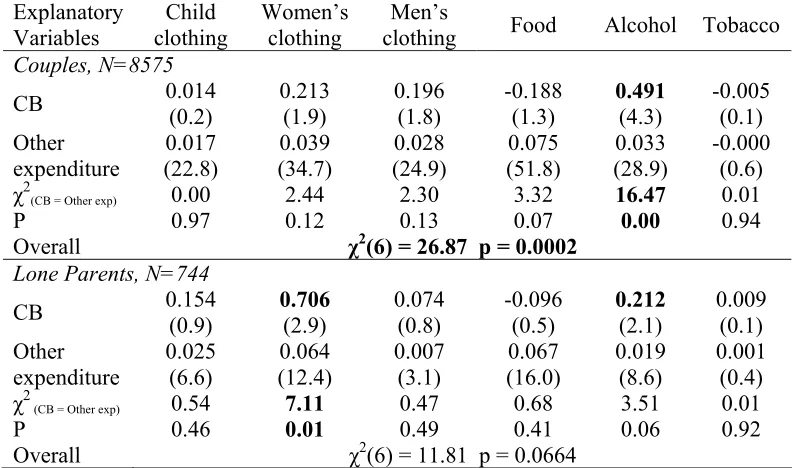
The benchmark results are shown in Table 3, which provides estimates using the couples and lone parents data for those with one child aged under 1634, who are not on welfare35. The assignable goods equations and the food equation are presented (the residual spending equation is not presented and the estimates are independent of the excluded equation). The coefficients show the effect of £1 of CB and of other income on spending on each good. The key result here is that it is alcohol spending that changes when CB changes with a marginal propensity of 0.49 for couples (0.21 for single parents) – much larger than the marginal propensity to spend on alcohol from other income. For lone mothers we find that there is a significant effect (0.71) on adult women’s clothing. In the case of couples the CB effect on alcohol, (and for lone parents the effect of CB on mother’s clothing) is more than ten times larger than the
33 We experimented with nonlinear Engel curves. For example, we found that when we entered CB and
other expenditure quadratically the marginal effects, evaluated at the means, were essentially unchanged. In any event we do go on to provide estimates for subsets of the data broken down by income and find that our main results carry over to each subset of the income distribution.
34 Results restricted to children under 11 are almost identical.
35 We investigated the sensitivity to including welfare recipients in the samples. For welfare recipients
Engel curve slope. The χ2 and P statistics test for the restriction that marginal propensity to spend out of CB income is the same as that out of other income (defined as total expenditure minus CB). The restriction that the marginal propensities to spend out of CB and other income are the same is rejected for alcohol in the couples sample, and for women’s clothing in the lone parent sample. The overall χ2 and P values test the restrictions, across all goods, that the effects of CB and other expenditure are the same. We strongly reject this restriction for couples although the value for lone parents is not quite significant36.
Table 3 Estimated effects of £1 of CB and £1 of other income on spending on each good: Parents with one child not on welfare, 1980-2000.
Explanatory
Variables clothing Child Women’s clothing clothing Men’s Food Alcohol Tobacco
Couples, N=8575
CB 0.014 (0.2) 0.213 (1.9) 0.196 (1.8) -0.188 (1.3) 0.491 (4.3) -0.005 (0.1) Other
expenditure (22.8) 0.017 (34.7) 0.039 (24.9) 0.028 (51.8) 0.075 (28.9) 0.033 -0.000 (0.6)
χ2(CB = Other exp) 0.00 2.44 2.30 3.32 16.47 0.01
P 0.97 0.12 0.13 0.07 0.00 0.94
Overall χ2(6) = 26.87 p = 0.0002
Lone Parents, N=744
CB 0.154 (0.9) 0.706 (2.9) 0.074 (0.8) -0.096 (0.5) 0.212 (2.1) 0.009 (0.1) Other
expenditure
0.025 (6.6)
0.064 (12.4)
0.007 (3.1)
0.067 (16.0)
0.019 (8.6)
0.001 (0.4)
χ2 (CB = Other exp) 0.54 7.11 0.47 0.68 3.51 0.01
P 0.46 0.01 0.49 0.41 0.06 0.92
Overall χ2(6) = 11.81 p = 0.0664
Note: Figures in parentheses are absolute t values. Other explanatory variables are: a linear trend; month, region and dummy variables for whether the child was aged 0-4, 5-10 or 11-15; a quadratic in age of household head; and a lone father dummy in the lone parent sample. The F statistic in each equation is a test of whether the coefficient on CB and on other income is equal, and the overall F statistic is a test that all of the CB coefficients equal the corresponding other income coefficients.
36 Clearly part of the variation in real CB arises because of differential inflation rates across years.
4.2 Robustness of Benchmark Results
Infrequency of purchase is clearly an issue in short survey datasets. This gives rise to a measurement error problem that would lead to biased estimates. Keen (1986) shows that this can be resolved by instrumenting total expenditure and here we use total household income as an instrument. Moreover, alcohol is well known to be under-reported in survey data. Since alcohol is a component of total expenditure then this would normally gives rise to the other income coefficient being biased towards zero. Under-reporting of spending on any good induces non-classical measurement error in total expenditure and, because of adding up it seems likely that bias will affect all equations. There do not appear to be any analytical results of the effects of this sort of measurement issue in the literature and there are no strong a priori grounds for thinking the bias should be systematically in one direction37.
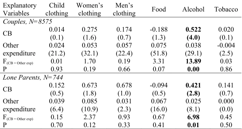
The results are reported in Table 4. In comparison with Table 3 there are some changes in magnitude but there is no change in the pattern or significance of results. In Table 5 we re-estimate using Tobit to allow for the zeroes in the expenditures. There is no change, relative to Table 3, for couples but for lone parents the result for women’s clothing becomes insignificant while alcohol becomes larger and significant. Thus, it seems unlikely that our results are driven by measurement error. If anything, our IV and Tobit results strengthen our conclusion from Table 3.
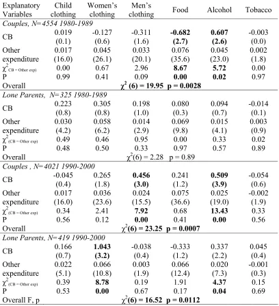
The identification of the CB coefficients in Table 3 derives entirely from the time series variation. While the real value of CB does not exhibit a time trend (and, in any event our modelling includes both a linear trend and a set of month controls) we first test for the robustness of the results in Table 3 by re-estimating over the 1980’s data (1980-1989) separately from the 1990’s (1990-2000) data. These results are presented in Table 6 for the 1980’s and the 1990’s separately. The results in Table 3 for the pooled data over the whole period are confirmed – with alcohol being the source of rejection for couples - men’s clothing in the latter period, and women’s clothing being the problem for lone mothers but only in the 1990’s. In Table 7 we re-
37 This instrument is commonly used in demand system estimation. See, for example, Blundell et al
Table 4 IV Estimates of Engel Curves: one child not on welfare, 1980-2000.
Explanatory
Variables clothing Child Women’s clothing clothing Men’s Food Alcohol Tobacco
Couples, N=8560
CB -0.011 (0.1) 0.152 (1.3) 0.158 (1.4) -0.309 (2.0) 0.434 (3.7) 0.000 (0.0) Other
expenditure (10.6) 0.006 (15.9) 0.014 0.008 (8.5) (29.0) 0.035 (16.3) 0.015 -0.003 (6.2)
χ2 (CB = Other exp) 0.05 1.38 1.72 4.74 12.99 0.00
P 0.83 0.24 0.19 0.03 0.00 0.96
Overall χ2(6) = 25.72 p = 0.0003
Lone Parents, N=738
CB 0.169 (0.9) 0.712 (2.7) 0.076 (0.8) -0.062 (0.3) 0.244 (2.3) 0.013 (0.2) Other expenditure 0.006 (2.1) 0.023 (5.6) 0.002 (1.5) 0.028 (7.9) 0.008 (4.8) -0.001 (0.7)
χ2(CB = Other exp) 0.81 6.95 0.54 0.16 4.94 0.03
P 0.37 0.01 0.46 0.69 0.03 0.86
Overall χ2(6) = 12.52 p = 0.0513
Note: Figures in parentheses are absolute t values. Other explanatory variables are: a linear trend; month, region, dummy variables for whether the child was aged 0-4, 5-10 or 11-15; a quadratic in age of household head; and a lone father dummy in the lone parent sample. Households with negative other incomes are excluded.
Table 5 Tobit Estimates of Engel Curves: one childnot on welfare, 1980-2000.
Explanatory Variables Child clothing Women’s clothing Men’s
clothing Food Alcohol Tobacco
Couples, N=8575
CB 0.014 (0.1) 0.275 (1.6) 0.174 (0.7) -0.188 (1.3) 0.522 (4.0) 0.020 (0.1) Other expenditure 0.024 (21.2) 0.053 (32.1) 0.057 (22.4) 0.075 (51.8) 0.038 (29.1) -0.004 (2.5)
F(CB = Other exp) 0.01 1.70 0.19 3.31 13.89 0.03
P 0.93 0.19 0.66 0.07 0.00 0.86
Lone Parents, N=744
CB 0.152 (0.5) 0.673 (1.8) 0.678 (1.0) -0.094 (0.5) 0.421 (2.8) 0.141 (0.7) Other expenditure 0.039 (6.4) 0.085 (10.9) 0.031 (2.3) 0.067 (16.0) 0.025 (8.1) 0.000 (0.0)
F(CB = Other exp) 0.15 2.37 0.93 0.67 6.98 0.45
P 0.70 0.12 0.33 0.41 0.01 0.50
[image:21.612.111.506.450.661.2]Table 6 Engel Curves: Parents with one child not on welfare: 1980-1989 and 1990-2000.
Explanatory Variables Child clothing Women’s clothing Men’s
clothing Food Alcohol Tobacco
Couples, N=4554 1980-1989
CB 0.019 (0.1) -0.127 (0.6) -0.311 (1.6) -0.682 (2.7) 0.607 (2.6) -0.003 (0.0) Other expenditure 0.017 (16.0) 0.045 (26.1) 0.033 (20.1) 0.076 (35.6) 0.045 (23.0) 0.002 (1.8)
χ2CB = Other exp) 0.00 0.67 2.96 8.67 5.72 0.00
P 0.99 0.41 0.09 0.00 0.02 0.97
Overall χ2 (6) = 19.95 p = 0.0028
Lone Parents, N=325 1980-1989
CB 0.223 (0.8) 0.305 (0.8) 0.198 (1.0) 0.080 (0.3) 0.094 (0.7) -0.014 (0.1) Other
expenditure 0.030 (4.2) 0.058 (6.2) 0.014 (2.9) 0.069 (9.8) 0.015 (4.1) 0.003 (0.9)
χ2(CB = Other exp) 0.49 0.46 0.95 0.00 0.33 0.02
P 0.48 0.50 0.33 0.97 0.57 0.89
Overall χ2(6) = 2.28 p = 0.89
Couples , N=4021 1990-2000
CB -0.045 (0.4) 0.265 (1.8) 0.456 (3.0) 0.241 (1.2) 0.509 (3.9) -0.054 (0.6) Other expenditure 0.017 (16.0) 0.036 (23.6) 0.024 (15.5) 0.075 (36.6) 0.025 (19.0) -0.002 (1.9)
χ2(CB = Other exp) 0.34 2.41 7.92 0.68 13.43 0.33
P 0.56 0.12 0.00 0.41 0.00 0.56
Overall χ2(6) = 23.25 p = 0.0007
Lone Parents, N=419 1990-2000
CB 0.166 (0.7) 1.043 (3.2) -0.038 (0.4) -0.333 (1.2) 0.337 (2.2) 0.045 (0.4) Other
expenditure 0.022 (5.1) (10.8) 0.066 0.003 (1.9) (12.4) 0.066 0.020 (7.3) -0.001 (0.3)
χ2(CB = Other exp) 0.39 8.78 0.19 1.91 4.37 0.15
P 0.53 0.00 0.67 0.17 0.04 0.69
Overall F, p χ2(6) = 16.52 p = 0.0112
Table 7 Engel Curves and Maternal Education: 1980-2000. Child clothing Women’s clothing Men’s
clothing Food Alcohol Tobacco
Mother left school at 16, Couples N=5271
CB 0.017 (0.2) 0.459 (3.4) 0.590 (4.6) -0.086 (0.5) 0.378 (2.8) 0.018 (0.2) Other expenditure 0.020 (18.2) 0.040 (27.8) 0.029 (21.1) 0.078 (39.6) 0.037 (26.1) 0.002 (1.9) χ2
(CB = Other exp) 0.00 9.65 18.75 0.78 6.43 0.02
P value 0.98 0.00 0.00 0.38 0.01 0.88
Overall χ2(6) = 32.15 p = 0.0000
Mother left school at 17/18, Couples N=1980
CB -0.146 (1.2) -0.017 (0.1) -0.129 (0.7) -0.246 (1.0) 0.579 (3.5) -0.013 (0.1) Other expenditure 0.016 (10.4) 0.043 (16.8) 0.026 (11.7) 0.074 (23.9) 0.030 (14.6) 0.003 (2.0) χ2
(CB = Other exp) 1.74 0.09 0.79 1.72 11.27 0.02
P value 0.19 0.77 0.37 0.19 0.00 0.88
Overall χ2(6) = 17.24 p = 0.0084
Mother left school at 19+, Couples N=1324
CB 0.543 (2.0) -0.042 (0.1) -0.377 (0.7) -0.710 (1.3) 0.892 (1.6) -0.014 (0.1) Other expenditure 0.016 (8.9) 0.035 (12.2) 0.029 (8.5) 0.068 (19.0) 0.031 (8.7) 0.001 (1.0) χ2
(CB = Other exp) 3.66 0.03 0.57 1.92 2.40 0.01
P value 0.06 0.86 0.45 0.17 0.12 0.91
Overall χ2(6) = 9.92 p = 0.1279
Mother left school at 16, Lone parents: N=366
CB 0.109 (0.6) 0.618 (2.4) -0.092 (1.2) -0.081 (0.3) 0.135 (1.2) 0.019 (0.2) Other
expenditure 0.054 (8.9) (11.5) 0.095 0.012 (5.2) (11.2) 0.086 0.022 (6.0) -0.000 (0.0) χ2
(CB = Other exp) 0.08 4.03 1.99 0.47 0.93 0.02
P value 0.78 0.04 0.16 0.49 0.33 0.88
Overall χ2(6) = 8.33 p = 0.2151
Mother left school at 17/18, Lone parents: N=154
CB 0.318 (0.5) 1.185 (2.1) 0.073 (0.4) -0.252 (0.6) 0.367 (1.5) 0.182 (1.1) Other expenditure 0.033 (3.3) 0.031 (3.3) 0.002 (0.6) 0.077 (10.7) 0.009 (2.2) 0.003 (1.2) χ2
(CB = Other exp) 0.22 4.29 0.17 0.59 2.19 1.23
P value 0.65 0.04 0.68 0.44 0.14 0.27
Overall χ2(6) = 8.03 p = 0.2357
Mother left school at 19+, Lone parents: N=224
CB 0.051 (0.2) 1.111 (2.0) 0.497 (1.9) -0.224 (0.5) 0.171 (0.7) -0.011 (0.1) Other expenditure 0.009 (1.7) 0.061 (6.3) 0.007 (1.5) 0.052 (7.0) 0.023 (5.6) 0.002 (0.8) χ2
(CB = Other exp) 0.02 3.67 3.59 0.44 0.41 0.01
P value 0.89 0.06 0.06 0.51 0.52 0.93
Overall χ2(6) =8.82 p = 0.1841
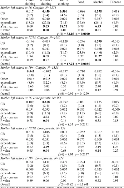
estimate for subsamples of mothers with different levels of education: left school at 16 (the minimum), at 17/18, or 19+. Our conclusion remains: couples reject through alcohol, while lone mothers reject through mother’s clothing.
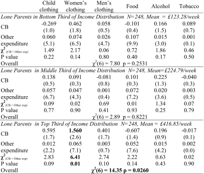
Tables 8a and 8b divides the samples into the top, middle and bottom thirds of the respective income (total expenditure) distributions. Again the headline results are broadly confirmed: all but the bottom third of couples significantly reject because of alcohol; while the top third of the lone mothers reject because of women’s clothing. Even for the bottom third the alcohol and women’s clothing coefficients on CB are much larger than the respective other income coefficients, albeit not significant.
Table 8a Engel Curves and Household Income:
Couples with one child not on welfare, 1980-2000.
Child
clothing Women’s clothing clothing Men’s Food Alcohol Tobacco
Couples in Bottom Third of Income Distribution N=2859, Mean inome = £215.81/week
CB 0.060 (0.4) 0.275 (1.3) 0.072 (0.4) -0.571 (1.8) 0.315 (1.4) 0.068 (0.4) Other expenditure 0.019 (12.9) 0.043 (20.0) 0.028 (13.8) 0.085 (27.0) 0.040 (17.8) 0.005 (2.8)
χ2(CB = Other exp) 0.08 1.18 0.05 4.43 1.54 0.12
P value 0.78 0.28 0.83 0.04 0.21 0.73
Overall χ2(6) = 7.95 p = 0.2415
Couples in Middle Third of Income Distribution N=2858, Mean income = £349.59/week
CB 0.094 (0.8) -0.017 (0.1) -0.132 (0.8) -0.016 (0.1) 0.348 (2.3) 0.035 (0.3) Other expenditure 0.018 (11.4) 0.036 (17.1) 0.030 (15.0) 0.067 (22.9) 0.023 (11.3) 0.004 (2.7)
χ2(CB = Other exp) 0.42 0.11 1.09 0.14 4.60 0.06
P value 0.52 0.74 0.30 0.71 0.03 0.80
Overall χ2(6) = 7.13 p = 0.3085
Couples in Top Third of Income Distribution N=2858, Mean income = £621.44/week
CB -0.086 (0.6) 0.343 (1.6) 0.508 (2.4) -0.184 (0.7) 0.701 (3.3) -0.036 (0.4) Other expenditure 0.016 (11.5) 0.038 (18.1) 0.027 (12.6) 0.065 (26.0) 0.031 (14.2) 0.001 (0.8)
χ2(CB = Other exp) 0.57 2.13 5.14 1.01 9.87 0.16
P value 0.45 0.14 0.02 0.31 0.00 0.69
Overall χ2(6) = 19.99 p = 0.0028
Table 8b Engel Curves and Household Income:
Lone Parents with one child not on welfare, 1980-2000.
Child clothing
Women’s clothing
Men’s
clothing Food Alcohol Tobacco
Lone Parents in Bottom Third of Income Distribution N=248, Mean = £123.28/week
CB -0.269 (1.0) 0.462 (1.8) 0.058 (0.5) -0.101 (0.4) 0.166 (1.5) 0.089 (0.7) Other
expenditure 0.060 (5.1) 0.074 (6.5) 0.026 (4.7) 0.107 (9.9) 0.015 (3.0) 0.001 (0.1)
χ2 (CB = Other exp) 1.49 2.17 0.06 0.72 1.86 0.46
P value 0.22 0.14 0.80 0.40 0.17 0.50
Overall χ2(6) = 7.80 p = 0.2531
Lone Parents in Middle Third of Income Distribution N=248, Mean=£224.79/week
CB 0.138 (0.5) 0.091 (0.3) -0.081 (0.8) 0.101 (0.3) 0.225 (1.3) -0.040 (0.3) Other
expenditure 0.057 (6.7) 0.047 (4.3) 0.001 (0.4) 0.072 (7.2) 0.020 (3.6) 0.003 (0.5)
χ2(CB = Other exp) 0.09 0.02 0.69 0.01 1.34 0.07
P value 0.77 0.90 0.41 0.93 0.25 0.79
Overall χ2(6) = 2.89 p = 0.8221
Lone Parents in Top Third of Income Distribution N=248, Mean = £416.85/week
CB 0.595 (1.7) 1.560 (2.6) 0.401 (1.7) -0.607 (1.4) 0.196 (0.9) -0.017 (0.1) Other
expenditure
0.012 (2.2)
0.065 (7.1)
0.003 (0.7)
0.052 (7.6)
0.015 (4.2)
0.002 (0.0)
χ2(CB = Other exp) 2.83 6.41 2.74 2.22 0.63 0.02
P value 0.09 0.01 0.10 0.14 0.43 0.90
Overall χ2(6) = 14.35 p = 0.0260
Note: Figures in parentheses are absolute t values. Other explanatory variables are: a linear trend; month, region and dummy variables for whether the child was aged 0-4, 5-10 or 11-15; and a quadratic in age of household head.
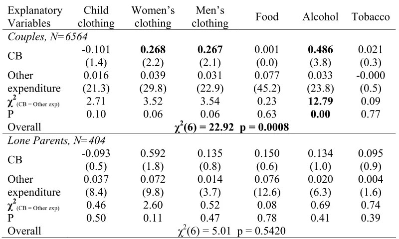
Table 9 replicates Table 3 but uses only the data for children under 11. We do this in case the benchmark results are contaminated by the possibility that parents may be wearing child clothing38. The strong results for couples remain although the precision of the lone mothers sample falls sufficiently that the effects become insignificant. Nevertheless the sizes of the coefficients for lone mothers are comparable with Table 3.
38 Although there is a sales tax distinction between adult and child clothing that is defined by sizes, the
Table 9 Engel Curves and Household Income: Child aged up to 10 only
Explanatory Variables
Child clothing
Women’s clothing
Men’s
clothing Food Alcohol Tobacco
Couples, N=6564
CB -0.101 (1.4) 0.268 (2.2) 0.267 (2.1) 0.001 (0.0) 0.486 (3.8) 0.021 (0.3) Other
expenditure
0.016 (21.3)
0.039 (29.8)
0.031 (22.9)
0.077 (45.2)
0.033 (23.8)
-0.000 (0.5)
χ2(CB = Other exp) 2.71 3.52 3.54 0.23 12.79 0.09
P 0.10 0.06 0.06 0.63 0.00 0.77
Overall χ2(6) = 22.92 p = 0.0008
Lone Parents, N=404
CB -0.093 (0.5) 0.592 (1.8) 0.135 (0.8) 0.150 (0.6) 0.134 (1.0) 0.095 (0.9) Other
expenditure 0.037 (8.4) 0.072 (9.8) 0.014 (3.7) (12.6) 0.076 0.020 (6.3) 0.004 (1.6)
χ2(CB = Other exp) 0.46 2.60 0.52 0.08 0.69 0.74
P 0.50 0.11 0.47 0.78 0.41 0.39
Overall χ2(6) = 5.01 p = 0.5420
Note: Figures in parentheses are absolute t values. Other explanatory variables are: a linear trend; month, region, dummy variables for whether the child was aged 0-4, 5-10 or 11-15; a quadratic in age of household head; and a lone father dummy in the lone parent sample. The F statistic in each equation is a test of whether the coefficient on CB and on other income is equal, and the overall F statistic is a test that all of the CB coefficients equal the corresponding other income coefficients.
4.3 Anticipated and Unanticipated Variation
Despite the weight of evidence here that suggests that variations in CB are reflected in adult-assignable, and not in spending on child-assignable, goods it would be inappropriate to conclude that the lack of equivalence between CB and other income implies that parents put less weight on the welfare of their children than on their own so that, at the margin, they favour expenditure on adult goods. Rather, an alternative explanation would be that parents may place so much weight on the welfare of their children that they fully insure them against income variations so that, at least unanticipated, variation in incomes does not affect spending on the children
Suppose the simplest case where all goods are exclusive to either adults or children and the utility function of the altruistic parent is defined as
(
)
(
)
a c
V y x− +αV x b+ where α>0 indicates altruism, y is the household income
(assumed to be the adult’s (a)), x is the transfer from parent to child (c), b is a transfer from the government to the child. Differentiating with respect to x shows that the
equilibrium transfer to the child is such that λa= −αλc (for an interior optimum
utilities of income. The optimal transfer, x*, is such that it would be the same if the welfare transfer, b, had been made to the parent rather than the child39. In the case where b is uncertain it is useful to consider a simple benchmark case of Va and Vc
being CRRA functions of y-x and x+b respectively. In this case the optimality property allows us to solve for x in terms of b. As before, the optimal x depends on the value of b but the size of the effect of b on x now depends on the ratio of the degrees of relative risk aversions and the extent of altruism. Only if the parents are sufficiently risk averse with respect to the child’s consumption, relative to their own consumption, and altruism is sufficiently large, will x vary inversely with b. In general, parents will not fully insure their children unless they themselves are risk neutral.
There is some qualitative evidence that suggests that parents (especially mothers) are likely to “go without” to protect spending on their children in the face of adverse shocks40. To investigate this issue we assume that households form static expectations of real CB. That is, we assume that households form rational expectations about the price level and so real CB falls within years according to the actual inflation rate; and we assume that between year changes the government will uprate nominal CB to be the same real level as at the previous uprating date. That is we assume that households assume that CB will be indexed in line with inflation since the last increase – and so have static expectations of policymakers. Thus, we decompose real child benefit according to the following formula:
(
)
12 12
ym
a
y y m y
CB =CB− P− P−
where CByma is the level of child benefit that would be anticipated in year y some m
months after the uprating, CBy-12 is the nominal value of CB at the last uprating and Py-m/Py-12 is the inflation adjustment over the last m months since the uprating. This
captures the variation in CB arising from the inflation that has occurred since the last uprating. The difference between actual CB and anticipated CB captures the change in CB that has occurred because of the nominal uprating that last occurred – which we
assume is unpredictable and call unanticipated CB,
ym
u
CB . We allow for there to be a
39 See Bergstrom (1989) for discussion of Becker’s rotten kid theorem.
40 Two recent examples of such work are Middleton, Ashworth, and Braithwaite (1997) and Farrell and
Table 10 Anticipated vs Unanticipated CB effects: Rational Expectations.
Couples, N=8575 clothing Kid’s Women’s clothing clothing Men’s Food Alcohol Tobacco
Anticipated CB -0.233 (1.3) 0.403 (1.5) 0.141 (0.5) -1.368 (3.9) 0.330 (1.2) 0.174 (1.1)
Unanticipated CB 0.066 (0.8) 0.173 (1.4) 0.208 (1.7) 0.059 (0.4) 0.524 (4.2) -0.043 (0.6)
Other expenditure (22.8) 0.017 (34.8) 0.039 (24.9) 0.028 (51.7) 0.075 (28.8) 0.033 -0.000 (0.6)
χ2(antCB= Other exp) 1.83 1.78 0.17 16.66 1.16 1.11
P 0.18 0.18 0.68 0.00 0.28 0.29
Overall χ2(6) = 23.84 p = 0.0006
χ2(unantCB= Other exp) 0.34 1.19 2.16 0.01 15.57 0.32
P 0.56 0.27 0.14 0.92 0.00 0.57
Overall χ2(6) = 20.06 p = 0.0027
Lone Parents N=744
Anticipated CB 0.085 (0.1) 0.775 (0.7) -0.079 (0.2) -0.326 (0.4) 0.323 (0.7) 0.143 (0.4)
Unanticipated CB 0.156 (0.9) 0.704
(2.9)
0.079
(0.8) -0.089 (0.4) 0.208 (2.0)
0.005 (0.1) Other expenditure 0.025 (2.4) (12.4) 0.064 0.007 (3.1) (16.0) 0.067 0.019 (8.6) 0.001 (0.4)
χ2(antCB= Other exp) 0.01 0.47 0.04 0.21 0.46 0.16
P 0.94 0.49 0.84 0.65 0.50 0.69
Overall χ2(6) = 1.28 p = 0.97
χ2(unantCB= Other exp) 0.55 6.93 0.53 0.61 3.31 0.00
P 0.46 0.01 0.46 0.44 0.07 0.96
Overall χ2(6) = 11.44 p = 0.0758
Note: Other expenditure is defined as total expenditure minus CB. Figures in parentheses are absolute t values. The lone parents equations include a dummy variable for lone father.
differential effect of these two components by writing our Engel curves as
+ + +
a u
ih i i i h h i ih
e = αCB γCB ηM Z β + ε where M is other expenditure. The results
are reported in Table 10 in the case where we assume that expectations of inflation are formed rationally.
on alcohol out of unanticipated CB is significantly different from spending out of other income, and for lone parents the same is true for both alcohol and women’s clothing. The F and P statistics show that in the couples sample the restriction that the marginal propensity to consume out of unanticipated CB is the same as that out of other income jointly for all equations is strongly rejected. However, the same restrictions cannot be rejected in the lone parent sample due to a smaller sample size and a lack of precision.
6. Conclusions
Our analysis finds that unanticipated variation in CB that is driven by policy induced changes in its real value is disproportionately spent on adult assignable goods. The results for couples suggest that, at the margin, more than a fifth (and perhaps as much as a half) of unanticipated changes in CB, is spent on alcohol. The results for lone parents are less strong but nonetheless still apparent. These findings contrast with those of Kooreman (2000), which exploits variation in Dutch CB, and of Edmonds (2002), based on data from Slovenia.
A weakness of this line of research is that it is unclear what inferences can be drawn from an equivalence (or lack of it) between CB and other income. One might be tempted to conclude that CB is treated differently because there is something different about it. For example, CB is usually given to the mother so that a lack of equivalence may suggest imperfect pooling of household incomes. However, our results are also true for lone parents where there is no intra-household distributional issue, so this cannot account for all of this lack of equivalence. It is true that the effect for lone parents is less pronounced, the alcohol coefficient for CB is around half the size as in the couples samples, and this is consistent with the idea that there is some free-riding between partners which does not occur in single parent households. A second issue might be that real CB variation tracks the business cycle implying that our results are attributable to cyclical effects in spending. However, we find no such cyclical effects in the spending patterns of households without children and there is little reason to expect households with children to differ in this respect.