Microarray BASICA: Background Adjustment,
Segmentation, Image Compression
and Analysis of Microarray Images
Jianping Hua
Department of Electrical Engineering, Texas A&M University, College Station, TX 77843, USA Email:[email protected]
Zhongmin Liu
Advanced Digital Imaging Research, 2450 South Shore Boulevard, Suite 305, League City, TX 77573, USA Email:[email protected]
Zixiang Xiong
Department of Electrical Engineering, Texas A&M University, College Station, TX 77843, USA Email:[email protected]
Qiang Wu
Advanced Digital Imaging Research, 2450 South Shore Boulevard, Suite 305, League City, TX 77573, USA Email:[email protected]
Kenneth R. Castleman
Advanced Digital Imaging Research, 2450 South Shore Boulevard, Suite 305, League City, TX 77573, USA Email:[email protected]
Received 14 March 2003; Revised 23 September 2003
This paper presents microarray BASICA: an integrated image processing tool for background adjustment, segmentation, image compression, and analysis of cDNA microarray images. BASICA uses a fast Mann-Whitney test-based algorithm to segment cDNA microarray images and performs postprocessing to eliminate the segmentation irregularities. The segmentation results, along with the foreground and background intensities obtained with the background adjustment, are then used for independent compression of the foreground and background. We introduce a new distortion measurement for cDNA microarray image compression and devise a coding scheme by modifying the embedded block coding with optimized truncation (EBCOT) algorithm (Taubman, 2000) to achieve optimal rate-distortion performance in lossy coding while still maintaining outstanding lossless compression performance. Experimental results show that the bit rate required to ensure sufficiently accurate gene expression measurement varies and depends on the quality of cDNA microarray images. For homogeneously hybridized cDNA microarray images, BASICA is able to provide from a bit rate as low as 5 bpp the gene expression data that are 99% in agreement with those of the original 32 bpp images.
Keywords and phrases:microarray BASICA, segmentation, Mann-Whitney test, lossy-to-lossless compression, EBCOT.
1. INTRODUCTION
The cDNA microarray technology is a hybridization-based process that can quantitatively characterize the relative abun-dance of gene transcripts [1,2]. Contrary to conventional methods, microarray technology promises to monitor the transcript production of thousands of genes or even the whole genome simultaneously. It thus provides a new and powerful enabling tool for genetic research and drug
image is obtained in which the pixel intensities reflect the level of mRNA expression. Usually a microarray image is shown RGB composite format, where the red and green channels correspond to the two channels of the microarray image obtained while the blue channel is set to zero. With the help of signal processing and data analysis operations such as ratio statistics, classification, and genetic regulatory net-work design, microarray images can shed light on the pos-sible regulation rules of transcription production sought by biologists and clinicians.
Microarray images cannot be used for genetic data anal-ysis directly. Appropriate image processing procedures are to be performed in order to extract information from the images for downstream analysis. Thousands of cDNA tar-get sites must first be identified as the foreground by an im-age segmentation algorithm. Then the intensity pair (R,G) that represents gene expression levels of both channels is extracted from every foreground target site with appropri-ate background adjustment. Subsequent data analysis is nor-mally conducted based on the log ratio logR/G of the in-tensity pair. As the very first step of cDNA microarray sig-nal processing, the accuracy of image processing is critical to the reliability of subsequent data analysis. Many image pro-cessing schemes have been developed for this purpose in re-cent years and can be found in various commercial and non-commercial software packages [3,4,5,6,7,8,9,10,11,12,
13,14,15,16,17,18,19]. Generally, because each channel of the microarray image is typically more than 15 MB in size, highly efficient compression is necessary for data backup and communication purposes. In order to save storage space and alleviate the transmission burden for data sharing, the search for good progressive compression schemes that provide suf-ficiently accurate genetic information for data analysis at low bit rates while still ensuring good lossless compression per-formance has become the focus of cDNA microarray image compression research recently [3,4,20].
This paper introduces a new integrated system called mi-croarray BASICA. BASICA brings together the image pro-cessing procedures required to accomplish the aforemen-tioned information extraction and data analysis, including background adjustment, segmentation, and compression. A fast Mann-Whitney test-based algorithm is presented for the initial segmentation of cDNA microarray images. This new algorithm can save up to 50 times the number of repetitions required from the original algorithm [5]. The resulting im-ages are then postprocessed to remove the segmentation ir-regularities. The segmentation results, along with the fore-ground and backfore-ground intensities, are saved into a header file for both data analysis and compression. A novel distor-tion measure is introduced to evaluate the accuracy of ex-tracted information. Based on this measure and the infor-mation provided by the header file, a new image compres-sion scheme is designed by modifying the embedded block coding with optimized truncation (EBCOT) algorithm [3], which is now incorporated in the JPEG2000 standard. Our experiments show that there appears to be no common bit rate that ensures sufficiently accurate gene expression data for different cDNA microarray images. On cDNA
microar-ray images of good quality, BASICA is able to provide from a bit rate as low as 5 bpp (bit per pixel) the gene expression data that are 99% in agreement with those of the original 32 bpp images.
2. DETAILS OF MICROARRAY BASICA
Microarray BASICA provides solutions to both processing and compression of cDNA microarray images. The major components of BASICA and their relationship with the el-ements of a microarray experiment are shown inFigure 1. Each two-channel microarray image acquired through the laser scanner is first sent to the segmentation component, where the target sites are identified. With the result of segmentation, the background adjustment component esti-mates each spot’s foreground and background intensities and calculates the log ratio values based on the background-subtracted intensities. After this, the calculated log ratio val-ues along with the segmentation information and other nec-essary data related to each spot are output for downstream data analysis. In the mean time, BASICA compiles the seg-mentation result and extracted intensities into a header file. With this header file, thecompressioncomponent encodes the foreground and background of both channels of the original image into progressive bitstreams separately. The generated bitstreams, plus the header file, are saved into a data archive for future access or are transmitted as shared data. On the other hand, to utilize the archived or transmitted data, BA-SICA can either quickly retrieve the necessary genetic infor-mation saved in the header file or reconstruct the microar-ray image with available bitstreams through the reconstruc-tioncomponent and redo the segmentation and background adjustment.
2.1. Segmentation with postprocessing
Segmentation is performed to identify the target sites in each spot where the hybridization occurs. In [8], various existing segmentation schemes are summarized and categorized into four groups: (1) fixed circle segmentation, (2) adaptive cir-cle segmentation, (3) adaptive shape segmentation, and (4) histogram segmentation.
Header file Progressive
bitstream Reconstruction
Segmentation Background
adjustment Data
analysis
Data sharing
Data archiving Compression
Header file Microarray
image
Data analysis Background
adjustment Segmentation
Figure1: The major units of BASICA.
position of the round region in each spot to cope with the misalignment.
Neither the fixed nor the adaptive circle segmentation can accommodate the variances in shape of the target sites in the images. To tackle this problem, more accurate and sophisticated segmentation methods are needed. The seg-mentation technique introduced in [8] uses seeded region growing [21], while other methods [5, 6, 10, 15, 17, 19] rely on more conventional histogram-based segmentation al-gorithms. The histogram-based methods generally compute a histogram of pixel intensities for each spot. Methods in [10,17,19] adopt a percentile-based approach, which sets the pixels in a high percentile range of the histogram as the fore-ground and those in a low range as the backfore-ground. Methods in [6,15] use a threshold-based approach. To ensure correct segmentation, methods in [10,15] employ repetitions to find the most stable segmentation. The histogram-based segmen-tation demonstrates good performance when a target site has a high hybridization rate, that is, a high intensity. However, the intensities of most target sites are actually very close to the local background intensities, and it is hard to segment correctly by finding a threshold based on the histogram only. In an attempt to solve this problem, Chen et al. introduced a Mann-Whitey test-based segmentation method in [5].
So far, no single segmentation algorithm can meet the demands of all microarray images. Segmentation algorithms are normally designed to perform well on microarray images acquired by certain type of arrayers and scanners. It is there-fore hard to compare them directly.
2.1.1. Mann-Whitney test-based segmentation In BASICA, we use the Mann-Whitney test-based segmenta-tion algorithm introduced by Chen et al. in [5]. The
Mann-Whitney test is a distribution-free rank-based two-sample test, which can be applied to various intensity distributions caused by irregular hybridization processes that are difficult to handle by conventional thresholding methods. Here we first give a brief description of the Mann-Whitney test-based segmentation algorithm.
Consider two independent sample sets X andY. Sam-ples X1,X2,. . .,Xm are randomly selected from set X, and Y1,Y2,. . .,Yn are randomly selected from set Y. All N = m+nsamples are sorted and ranked. DenoteRias the rank of theith sample,R(Xi) as the rank of sampleXi, andR(Yi) as the rank ofYi. These ranks are used to test the following hypotheses:
(H0) P(X < Y)≥0.5, (H1) P(X < Y)<0.5.
Define the rank sum of themsamples fromXas
T= m
i=1
RXi. (1)
To avoid deviations caused by ties,T is commonly normal-ized as
T= T−m
(N+ 1)/2
nm/N(N−1)Ni=1Ri2−nm(N+ 1)2/4(N−1) . (2)
Hypothesis (H0) will be rejected ifTis greater than a certain quantilew1−α, whereαis the significance level.
hypothesis (H0) corresponds to the reverse case. To segment a target spot, a predefined target mask (obtained by select-ing, unifyselect-ing, and thresholding strong targets) is first applied to the spot. Pixels inside the mask correspond to setX, and pixels outside correspond to setY. To start the test,n sam-ples are randomly selected from setY, whilemsamples with lowest intensities are selected from setX. If hypothesis (H0) is accepted, the pixel with lowest intensity is removed from setX, andmsample pixels are reselected. The test is repeated until hypothesis (H0) is rejected. Then the pixels left in setX are considered as the foreground at significance levelα. The foregrounds obtained from the two channels are united into one to produce the final segmentation result.
The repetitive nature of this algorithm makes it cumber-some for real-time implementation. So, in BASICA, we pro-posed a fast Mann-Whitney test-based algorithm [3] which runs much faster while generating identical segmentation re-sults.
2.1.2. Speeding up Mann-Whitey test-based segmentation algorithm
Assume that the predefined target mask is obtained accord-ing to the way described in [5, 6]. Samples X1,X2,. . .,Xm andY1,Y2,. . .,Ynare picked from the foreground and back-ground, respectively. Without loss of generality, it suffices to assume thatX1≤X2≤ · · · ≤XmandY1≤Y2≤ · · · ≤Yn. SinceX1,X2,. . .,Xm are the smallestmsamples in setX, all other samples can be determined if X1 is set. Then Mann-Whitney test-based segmentation is actually an optimization problem of minimizingX1subject toT≥w1−α. Chen et al.’s approach takes a large number of repetitions to reach the fi-nal segmentation. However, it turns out that the number of repetitions can be significantly reduced by carefully choosing the starting point and search strategy.
BASICA first finds an upper bound of the optimal X1, denoted byXmax the average of those ranks if there would have been no tie, and induce a reduction on the sum. A property of this reduc-tion is that it is only related to the number of samples tied at that value. If there areksamples having the same value, the deduction is (1/12)(k3−k). With this property, one can easily reduce the upper bound ofNi=1R2i. Assume that∆Y is the decrease in the sum caused by the ties in the sorted Y1,Y2,. . .,Yn, then we have among themselves and share no tie with any sample in Y1,Y2,. . .,Yn. In most cases, the difference is very small and the bound is quite tight.
To simplify the notation, we useσmaxto denote
ThenX1maxmust satisfy the inequality
m is to find the smallestX1 so that the smallest rank sum of
X1≤X2≤ · · · ≤Xmstill satisfies inequality (6). To associate
Thus, the upper boundX1maxis the smallest sample inX that is larger thanYu. For any sample setX1,X2,. . .,Xmwith X1 ≥ X1max, hypothesis (H0) can be rejected outright. Since X1,X2,. . .,Xmnormally have similar intensities which bring on consecutive ranks,Xmax
1 is very close to the actual thresh-old. Hence, the repetitions can be greatly reduced if backward repetitions based onX1maxare applied.
Besides changing the starting point and repetition direc-tion, a two-tier repetition strategy can be used to reduce the repetition in case the upper bound is not so tight as expected. In the first tier, one does not perform the repetition in a pixel-by-pixel manner, but in a leaping manner instead. Then a pixel-by-pixel repetition follows up and locates the exact seg-mentation in the second tier. Larger step size means fewer repetitions in the first tier but more in the second, while smaller step size has the opposite effect. A natural choice of the repetition steps is indicated byY1,Y2,. . .,Ynwhennis not very large. The whole algorithm is described as follows.
Step 1: Calculateuusing (7).
Step 2: Find the smallestmsamples from setXthat are larger thanYu, and execute the Mann-Whitney test. Step 3: If hypothesis (H0) is rejected, then setu=u−1 and go to step 2, otherwise, go to step 4.
Step 4:u=u+ 1. Find the smallestmsamples from set Xthat are larger thanYu, and begin the pixel-by-pixel repetition in backward manner.
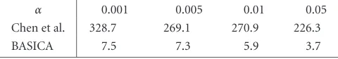
Table1: The comparisons of the number of repetitions between Chen et al.’s algorithm and our modified method used in BASICA at different significance levels.
α 0.001 0.005 0.01 0.05
Chen et al. 328.7 269.1 270.9 226.3
BASICA 7.5 7.3 5.9 3.7
to obtain identical results, the backward-searching nature of the new algorithm requires the normalized rank sum in (2) to be strictly increasing during the repetition of the origi-nal algorithm. This is not guaranteed due to the occurrences of ties in the sorted samples. In one extreme case, when all N samples have the same intensity, the devisor will become zero and the normalized rank sum will be infinity. Actually, Chen et al.’s original algorithm can be viewed as trying to find the largest foreground that rejects hypothesis (H0), while the modified algorithm in BASICA tries to find the smallest fore-ground that accepts the hypothesis H0. Since in most cases the normalized rank sum will be strictly increasing, we ex-pect the segmentation results of the modified algorithm to be identical to the original algorithm most of the time.
The comparisons of the number of required repetitions between Chen et al.’s algorithm and our modified algorithm are given inTable 1. Results are averaged over 504 spots in both channels from different test images. Both algorithms set m=n=8 and use the same randomly selected samples from the predefined background for the Mann-Whitney test. We find that the segmentation results on all test spots of the sam-ple images used in this study are identical between the orig-inal algorithm and the modified algorithm. From the table, we observe that the modified algorithm reduces the number of repetitions by up to 50 times from what is required of the original algorithm.
2.1.3. Postprocessing
Like common threshold-based segmentation algorithms, there are always many annoying shape irregularities in the segmentation results obtained by the Mann-Whitney test-based algorithms. These irregularities occur randomly and can severely reduce the compression efficiency. Thus, an ap-propriate postprocessing procedure is necessary to achieve efficient compression. Moreover, because most irregularities are pixels with a high probability of noise corruption, elimi-nating them is unlikely to compromise the accuracy of sub-sequent data extraction and analysis.
In BASICA, we categorize possible irregularities into two types and employ different methods to eliminate them. The first type includes isolated noisy pixels or tiny regions, which can be observed from the lower half of the segmentation result in Figure 2a. These irregularities are caused usually by nonspecific hybridization or undesired binding of fluo-rescent dyes to the glass surface. The second type includes the small branches attached to the large consolidated fore-ground regions, which are visible in the segmentation results ofFigure 2. Since these irregularities are located between the
foreground and background, their intensities are also inbe-tween, making them vulnerable to noise corruption. The ir-regularities in most segmentation results are usually made up of both these two types. For the first type, BASICA will detect and remove them directly from the foreground. As for the second type, BASICA applies an operation similar to the standard morphological pruning [22]. By removing and pruning repetitively, BASICA can successfully eliminate most irregularities in three to five repetitions. The right column of
Figure 2shows the postprocessing results on the original seg-mentation which are to be used for the compression of the images.Figure 3shows a portion of a microarray image and its segmentation results.
2.2. Background adjustment
It is commonly believed that the pixel intensity of the fore-ground reflects the joint effects of the fluorescence and the glass surface. To obtain the expression level accurately, the intensity bias caused by the glass surface should be esti-mated and subtracted from the foreground intensity, and this process is known as background adjustment. Since there is no hybridization in the background area, the background intensity is normally measured and treated as an intensity bias. Although mean pixel intensity has been adopted in al-most all existing schemes as the foreground intensity, sev-eral methods have been developed for background inten-sity estimation. The major differences of various methods lie in two aspects: (1) on which pixels the estimation is based and (2) how to calculate the estimation. Regarding the first aspect, the regions chosen for background estimation vary from a global background to a local background. For the global background, the background regions in all spots are considered, and a global background intensity is estimated and subtracted from every foreground intensity [9,16]. The global background ignores possible variance between sub-arrays and spots. So, in [9], partial global background esti-mation is performed based on the background of one subar-ray or on several manually selected spots. The more common approach is to estimate the background intensity based on the local background for each target site separately. The local background can be the entire background region in one spot [18], or, to avoid interference from the foreground, it can be the region with a certain distance from the foreground tar-get site [7,11,13,15,17]. In the extreme case, the algorithm in [14] uses the pixels on the border of each spot as the lo-cal background. However, using too few pixels increases the possibility of a large variance in background estimation. As to the second aspect, almost all existing systems adopt mean or median to measure the expression level. Besides these, mode and minimum are also used in some softwares [6,16]. Unlike all the methods mentioned above, a morphological opening operation is performed in [8] to smooth the whole back-ground and then estimate the backback-ground by sampling at the center of the spot.
(a)
(b)
Figure2: Segmentation and postprocessing of two typical spots. The left column shows the original microarray spots in RGB composite format. Some intensity adjustments are applied in order to show them clearly. The middle column shows the corresponding segmenta-tion results using the Mann-Whitney test with significance levelα =0.001. The right column shows the final segmentation results after postprocessing.
(a) (b)
Figure3: (a) Part of a typical cDNA microarray image in RGB com-posite format. Some intensity adjustments were applied in order to show the image clearly. (b) The segmentation results of (a).
provides seven ways of background region determination and six choices of averaging method. Experiments in [8] show that different background adjustment methods have significant impact on the log ratio values subsequently ob-tained. However, there is no known criterion to measure which approach is more accurate than the others.
BASICA chooses the average of pixel intensities in the lo-cal background as the estimate of background intensity. To prevent possible biases caused by either the higher intensity values of the pixels adjacent to the foreground target sites or the lower intensity values of the dark hole regions in the mid-dle of the spots, the local background used in BASICA is the background defined by the predefined target mask obtained through the segmentation.
2.3. Data analysis
Because so many elements impact the pixel intensities of the microarray image, genetic researchers do not use the absolute intensities of the two channels, but the ratio between them to measure the relative abundance of gene transcription. Not all genetic information extracted are reliable enough for data analysis. If the spot has so poor quality that no reliable infor-mation can be extracted, it is qualified as a false spot; other-wise, it is a valid spot. For a valid spotk, the expression ratio is denoted by
Tk=RkGk = µFRk−µBRk µFGk−µBGk
, (8)
andµBGkare the respective estimated background mean in-tensities. Because expression ratio has an unsymmetric dis-tribution, which contradicts the basic assumptions of most statistic tests, the log ratio logTk =logRk/Gkis commonly used instead in most applications. In addition to the log ra-tio, an auxiliary measure which is often helpful in data anal-ysis is the log product logRkGk. However, since the log trans-form does not have constant variance at different expres-sion levels, some alternative transforms like glog [23] have recently been introduced. In gene expression studies, such transformed ratios are ordinarily normalized and quantized into three classes: down-regulated, up-regulated, and invari-ant. Expression level extraction and quantization provide the starting point for subsequent high-level data analysis, and their accuracy is crucially important. Therefore, compres-sion schemes should be designed to minimize the distortion in the image, and their performance should be assessed by agreement/disagreement in gene expression level measure-ment caused by the compression. These topics will be dis-cussed in detail in Sections2.4and3.3.
2.4. Image compression
Since microarray images contain huge amounts of data and are usually stored at the resolution of 16 bpp, a two-channel microarray image is typically between 32 and 64 MB in size. Efficient compression methods are highly desired to accom-modate the rapid growth of microarray images and to reduce the storage and transmission costs. Currently, the common method to archive microarray images is to store them loss-lessly in TIFF format with LZW compression [24]. However, such an approach does not exploit 2D correlation of data be-tween pixels and does not support lossy compression. Due to the huge data size, microarray images require efficient pression algorithms which support not only lossless com-pression but also lossy comcom-pression with graceful degrada-tion of image quality for downstream data analysis at low bit rates.
Recently, a new method known as the segmented LOCO (SLOCO) was introduced in [20]. This method exploits the possibility of lossy-to-lossless compression for microarray images. SLOCO is based on the LOCO-I algorithm [25], which has been incorporated in the lossless/near-lossless compression standard of JPEG-LS. SLOCO employs a two-tier coding structure. It first encodes microarray images loss-ily with near-lossless compression, then applies bit-plane coding to the quantization error to refine the coding results until lossless compression is achieved. SLOCO can generate a partially progressive bitstream with a minimum bit rate de-termined by the compression of the first tier, and the coding is conducted on the foreground and background separately.
In BASICA, we also incorporate lossy-to-lossless com-pression of microarray images. The aims of comcom-pression in BASICA are twofold: (1) to generate progressive bitstreams that can fulfill the requirements of signal processing and data analysis at low bit rates for data sharing and transmission ap-plications and (2) to deliver competitive lossless compression performance to data archiving applications with a
progres-sive bitstream. To achieve these objectives, the compression scheme in BASICA treats the foreground and background of microarray images separately. Obviously, the foreground and background usually have significant intensity differences and they are relatively homogeneous in their corresponding lo-cal regions. Hence, by compressing the foreground and back-ground separately, the compression efficiency is expected to improve significantly. This is done by utilizing the outcomes of segmentation. Before encoding, BASICA saves all neces-sary segmentation information into a header file for subse-quent compression.
SLOCO in [20] is based on spatial domain predictive coding. In contrast, BASICA employs bit-plane coding in the transform domain. Bit-plane coding enables BASICA to achieve truly progressive bitstream coding at any rate. To al-low lossy compression, an appropriate distortion measument is needed. Generally, medical image compression re-quires visually imperceptible differences between the lossily reconstructed image and the original. Traditional distortion measures, such as mean square error (MSE), are poor indica-tors for this purpose. However, unlike other types of medical images, the performance of microarray image compression does not depend on visual quality judgement, but instead on the accuracy of final data analysis. Therefore, it is reasonable to adopt a distortion measure adherent to the requirements of data analysis. Since almost all existing data analysis meth-ods use the transformed expression values, we should seek to minimize the distortion under these measurements. In BA-SICA, we adopt distortion measures based on the log ratios and the log products because they are the most used trans-forms in common applications. However, as we will see later, the scheme employed in BASICA can be easily adapted for other transform measures.
The log ratios and the log products decouple the data of two channels into two separate log intensities, logRand logG. This ensures that the compression can be done on each channel independently. Without loss of generality, we only refer to theRchannel in the rest of the paper.
BASICA currently employs the MSE of logRas the dis-tortion measurement, which is defined as
MSElogR=N1
whereNis the total number of spots in the microarray image, andRi and ˆRi are background-subtracted mean intensities obtained from spotiof the original and reconstructed image, respectively.
There is a direct relationship between the MSE of log in-tensity and the traditional MSE. For spotk, its log intensity logRkcan be further written as
logRk=logµFRk−µBRk
∆logRkis associated with the unit error∆Xjof jth pixel by
∆logRk=M ∆Xj kµFRk−µBRk
. (11)
For the pixels in the background, because most existing schemes do not compute the average intensity asµBRkbut use nonlinear operations such as modulo or median filtering, the above derivation no longer holds. The foreground and back-ground pixels have different impacts on the log intensity and should be considered separately.
Equation (11) indicates that the MSE of log intensity is actually a weighted version of traditional MSE. The weight 1/Mk(µFRk−µBRk) is a constant for pixels in the same spot and is inversely proportional to the spot’s intensity and fore-ground size. The higher a spot’s intensity or forefore-ground size, the larger its allowable reconstruction error.
Quite similarly, one can easily derive other MSE distor-tion measurements for other transforms. For example, the glog transform in [23] is
whereαandcare parameters estimated from the microarray image. Then, with straightforward derivation, one can asso-ciate the unit error∆g(Rk) with the unit error∆Xj of jth
Thus, the MSE ofglog is also a weighted version of tradi-tional MSE, and like MSE of log ratio, the measurement al-lows larger distortions in spots of high intensities.
Although we can derive different distortion measure-ments for different transforms, the compression scheme in BASICA can only be designed based on one type of distortion measurement. As mentioned before, in BASICA we choose MSE of log ratio as the distortion measurement.
With the help of (11), we introduce a new lossy-to-lossless compression scheme in BASICA by modifying EBCOT [26] with several techniques specifically designed for the requirements of microarray technology. First, to encode the foreground and background separately, we modify the EBCOT to compress arbitrarily shaped regions. Then we ap-ply intensity shifts and bit shifts on the coefficients to mini-mize the MSE of log intensity.
EBCOT, which is a state-of-the-art compression algo-rithm incorporated in JPEG2000 standard, offers a fully pro-gressive bitstream of excellent compression efficiency with plenty of useful functionalities. In EBCOT, a 2D integer wavelet transform is applied for lossy-to-lossless image com-pression. Block-based bit plane coding is used to generate the bitstream of each subband. To achieve the optimal rate-distortion performance, the coding procedure consists of three passes in each bit plane using three context modeling
primitives. The bitstreams of all subbands are multiplexed into a layered one via a fast bisectional search for the given target bit rate.
2.4.1. Modifying EBCOT for microarray image coding
Our major modifications to EBCOT are the following.
Header file.A header file is necessary for saving the in-formation which will be used in the encoding and decod-ing procedures. To ensure that the encoder and decoder can correctly compress and reconstruct the foreground and background independently, the segmentation information must be saved in the header file. Besides, (11) indicates that the mean intensities of the foreground and background are also needed by the compression algorithm. To save storage memory, these data are coded with LZW compression. Al-though the segmentation information and spot intensities are enough for the compression component, other data, such as variances of pixel intensities in each spot, can also be saved in the header file for quick genetic information retrieval. In the practical implementation, the header file will be gener-ated before encoding and must be transmitted and decoded first.
Shape-adaptive integer wavelet transform. Like other frequency-domain-based coding schemes, in BASICA the transform is performed before bit-plane coding during the encoding phase and after the bit-plane reconstruction dur-ing the decoddur-ing phase. To ensure lossless compression, inte-ger wavelet transforms are required. The wavelet transforms are conducted on the foreground and background indepen-dently to prevent any interference between the coefficients from adjacent areas. Since the segmented foreground and background always have irregular shapes, critically sampled integer wavelet transforms for arbitrarily shaped objects are needed to ensure coding efficiency. Many approaches have been proposed for 2D shape-adaptive wavelet transforms. Our proposed coding scheme uses odd-symmetric exten-sions over object boundaries described in [27].
Object-based EBCOT. After shape-adaptive integer wavelet transform, we modify the EBCOT context modeling for arbitrarily shaped regions. The extension of EBCOT algorithm to shape-adaptive coding is rather straightfor-ward. Because the shape-adaptive integer wavelet transform is critically sampled, the number of wavelet coefficients is the same as those in the original regions. Using the wavelet-domain shape mask, one can easily tell whether a coefficient belongs to a region to be coded. If any neighbor of that coefficient falls outside the region, we just set that neighboring coefficient’s values to zero, thus making it insignificant in context modeling. We call the resulting coder object-based EBCOT.
in the foreground of any spotknormally have similar intensi-ties and roughly have a symmetric distribution aroundµFRk. So, for the encoding of the foreground, each pixel in spot k is subtracted µFRk instead of the global average intensity. SinceµFRk is already saved in the header file, intensity shifts do not cost any overhead. With intensity shifts, the distribu-tion of foreground intensities are transformed into a sym-metric shape with a high peak around zero. As for the back-ground compression, through our experiments, we find that the pixels in the background actually have a roughly symmet-ric intensity distribution, suggesting that the global average intensity subtraction will be appropriate.
Bit shifts.EBCOT uses block-based bit-plane coding. In order to minimize the distortions at different rates, one must code the bit planes of different spots according to their im-pacts on the MSE of log intensity. One straightforward solu-tion is to scale the coefficients of each spot with the spot’s weight, so bits at the same bit plane of all spots have the same impacts on the MSE of log intensity. However, because the weights are noninteger fractions, lossless compression cannot be ensured under such a scaling. Furthermore, al-though one can round them to the closest integer as an ap-proximation, any scalerwwill increase a coefficient’s infor-mation up to log2w bits, which can lead to a very poor lossless compression performance. In BASICA, we apply the scaling by bit shifts, which is a good approximation and meanwhile does not compromise the performance of lossless compression. For spotk, BASICA obtains
Sk=log2MkµFRk−µBRk
+ 0.5. (14)
LetSmax=max{S1,S2,. . .,S
N}. Then it scales the coefficients of spotkby upshifting themSmax−S
kbits.
Background compression.With careful consideration, bit shifts have not been applied in the background compression in BASICA for several reasons. First, since there exist diff er-ent approaches to compute the background intensity, and the values obtained by these methods also vary a lot, it is unclear how to find a unique weight for each pixel like what BASICA has for foreground compression. Second, unlike isolated tar-get sites in the foreground, the local background is normally connected to each other. Thus, bit shifts will bring abrupt in-tensity changes along the borders of spots, which will in turn lower the compression efficiency significantly in lossless cod-ing performance. Even though one can figure out the weights through a formula similar to (11) based on certain back-ground extraction methods, there will be a significant trade-offon lossless compression, which is about 0.8 bpp according to our experiments. So, in BASICA, we apply a global aver-age intensity subtraction and no bit shifts on the background compression, that is, the traditional MSE measure is used for rate-distortion optimization. Normally, the pixel inten-sities in the background are located in a very small range, which means that the background is pretty homogenous. Thus, compression with traditional MSE measure should be able to represent the background with fairly small bit rates.
To this end, the final code of a two-channel microarray image is composed of five different parts: a header file and
two bitstreams representing the foreground and background, respectively, from each channel.
3. EXPERIMENTAL RESULTS AND DISCUSSION
Experiments have been conducted to test the performance of BASICA with eight microarray images from two different sources. We used three test images from the National Insti-tutes of Health (NIH). Each of these images contains eight subarrays arranged in 2×4 format. In each subarray, the spots are arranged in a 29×29 format. There are a total of 20184 spots in all the three NIH images. In addition to these, we also tested on another set of five test images obtained from Spectral Genomics Inc. (SGI). Each of the SGI images con-tains eight subarrays arranged in 12×2 format, and in each subarray, the spots are arranged in a 16×6 format. These five SGI images contain a total of 9960 spots. The target sites in the NIH images exhibit noticeable irregular hybridization effect and have irregular brightness patterns across the spots. The intensities of these target sites span over a large range and vary considerably. The target sites in the SGI images appear to be hybridized more homogeneously, and many of them have nearly perfect circular shape.
In the experiments, for each two-channel image, the summed bit rate of all the bitstreams from both channels, plus the shape information, were reported in bpp format, which represents either the compression bit rate or the recon-struction bit rate, depending on the type of test performed. And the corresponding bit rate of the uncompressed original image is 32 bpp. BASICA first segmented the image and gen-erated the header file. The average overhead of the header file was 0.5 bpp for the NIH images and 0.24 bpp for the SGI im-ages, based on the postprocessed segmentation results. The header file overheads were smaller on the SGI images because of different settings of the microarray arrayers used to ac-quire the images: there were much fewer spots in each SGI image than those in each NIH image. After generating the header file, the foreground and background of each channel were compressed independently.
3.1. Comparisons of wavelet filters and decomposition levels
The framework of the proposed compression scheme in BA-SICA does not specify which wavelet filters and how many wavelet decomposition levels used. In order to find the op-timal choice for microarray image compression, we com-pare the results generated with different wavelet filters and decomposition levels. All the results presented in this section are based on the NIH images unless stated otherwise.
Table2: Lossless compression results (in bpp) of BASICA using different integer wavelet filters with one-level wavelet decomposition. The results are averaged over the NIH images.
Wavelet filters 9/7−F (2 + 2, 2) 5/3 S+P (4,2) (2,4) (4,4) (6,2) 2/6
File size 13.99 14.01 13.97 14.03 14.01 13.97 13.99 14.04 14.00
Table3: Lossless compression results (in bpp) of BASICA using the 5/3 wavelet filters with different wavelet decomposition levels. The results are averaged over the NIH images.
Decomposition levels 1 level 2 levels 3 levels 4 levels 5 levels File size 13.97 14.00 14.01 14.02 14.02
discrepancies in the results were small, the choice of the wavelet filters appeared to be not critical to the system per-formance.
Table 3 lists the lossless coding results by BASICA with different wavelet decomposition levels. Only the best-performing 5/3 wavelet filters were evaluated in these tests. The performance appeared to get worse when the decompo-sition level increased and compression with only one-level decomposition achieved the best result. This is partly due to the fact that although with more decompositions more data energy is compacted into smaller subbands, it also introduces a higher model-adaptation cost to arithmetic coding in the newly generated subbands, which cancels out the gains. Sim-ilar to the comparison among the wavelet filters, the discrep-ancies of lossless compression performance using different decomposition levels are very small. To confirm this obser-vation, lossy compression tests were also performed to com-pare the performances based on the choices of the wavelet decomposition level.
To evaluate the effect of lossy compression on data anal-ysis, the test images were first reconstructed at a target rate. Then the reconstructed images were processed and genetic information (i.e., log ratio) was extracted and compared with the same information extracted from the original images. To ensure credibility of the comparisons, the Mann-Whitney test-based segmentation started with the same selection of random pixels in the predefined background in both the re-constructed image and the original image. The segmenta-tion was conducted under three different significance levels α =0.001, 0.01, and 0.05. At each significance level, log ra-tios were extracted and distortions were computed. The dis-tortions shown are the average disdis-tortions at the three signif-icance levels over the three test images. Both thel1distortion andl2distortion (i.e., MSE) of log intensity were used as the error measures. Figure 4 shows the average reconstruction errors using BASICA at different bit rates with three diff er-ent decomposition levels of the 5/3 wavelet transform. From this figure, we can see that one-level decomposition yielded a significantly better performance than the others. Based on the above lossless and lossy compression results, we decided to use the 5/3 wavelet filters with one-level wavelet decom-position as a default setting in BASICA.
3.2. Comparisons of lossless compression
We first compared the lossless compression performance of BASICA with three current standard coding schemes: TIFF, LS, and JPEG2000. In the comparisons, TIFF, JPEG-LS, and JPEG2000 all compress a microarray image as a sin-gle region and no header file is added. To evaluate the im-provement brought by the postprocessing in segmentation, along with the intensity and bit shifts in compression, we also performed the tests of BASICA without the intensity and bit shifts and without postprocessing, respectively (denoted by BASICA w/o PP and BASICA w/o shifts, respectively, in Figures5,6, and7, andTable 4).
The coding results are shown inTable 4. The TIFF for-mat, which is commonly used in existing microarray im-age archiving systems, produced the poorest results, about 4 bpp worse than all the other methods compared. JPEG-LS achieved the best performance on the NIH images. But like TIFF, it does not support lossy compression. The proposed BASICA turned out to be about 0.27 bpp worse than JPEG-LS on the NIH images and 0.12 bpp better on the SGI images. Besides, BASICA was significantly better than JPEG2000 with the savings of 0.48 bpp and 0.56 bpp on the NIH and SGI images, respectively. BASICA with-out intensity and bit shifts yielded almost the same per-formance as BASICA in lossless compression. On the other hand, one can see clearly that the irregularities in segmen-tation reduced compression efficiency substantially. With-out postprocessing, the average size of a header file was 0.33 bpp larger than that of BASICA on the NIH images and 0.09 bpp larger on the SGI images, respectively. Thus, BA-SICA with postprocessing was preferred on all the test im-ages.
3.3. Comparisons of lossy compression
During the experiments, we also compared the lossy com-pression results at different bit rates. Since TIFF and JPEG-LS do not support the lossy compression functionality, JPEG2000 was the only standard compression scheme com-pared in the experiments. Our comparisons were based on three different measurements.
3.3.1. Comparisons based onl1andl2distortions
1-level 2-level 3-level
Reconstruction bitrate (bpp)
2 3 4 5 6 7 8 9 10 11
0 0.05 0.1 0.15 0.2 0.25 0.3 0.35
l1
dist
o
rt
ion
o
f
log
ra
tio
(a)
1-level 2-level 3-level
Reconstruction bitrate (bpp)
2 3 4 5 6 7 8 9 10 11
0 0.05 0.1 0.15 0.2 0.25
l2
dist
o
rt
ion
o
f
log
ra
tio
(b)
Figure4: Rate-distortion curves of log ratio in terms of (a)l1distortion and (b)l2distortion with different wavelet decomposition levels
at different reconstruction bit rates; 5/3 wavelet filters were used. The segmentation was performed at three different significance levels,
α = 0.001, 0.01, and 0.05, and three log ratios and their corresponding distortions were then obtained. The distortions shown are the averages of the three significance levels over the NIH images.
Table4: Lossless compression results (in bpp) of different coding schemes.
Methods TIFF JPEG-LS JPEG2000 BASICA w/o shifts BASICA w/o PP BASICA
Bit rates (NIH) 18.27 13.70 14.45 13.99 14.50 13.97
Bit rates (SGI) 17.21 14.49 14.93 14.31 14.46 14.37
low bit rates, only inferior to BASICA on the NIH images and similar to the others on the SGI images. Nevertheless, it pro-duced relatively largel2distortion values. Apparently, with-out adjusting the MSE for log intensity, JPEG2000 spent too many bit rates on high-intensity pixels/spots, which led to highl2distortion. Furthermore, the distortion of JPEG2000 decayed slowly in bothl1andl2senses. For bit rates beyond 6 bpp, it degraded to produce the worst distortion among all the methods. Without the intensity and bit shifts, BASICA performed poorly at lower bit rates. Only when the bit rates went above 6 bpp did its performance become acceptable. BASICA without postprocessing produced different perfor-mances on images of different sources. On the NIH images, it obviously suffered from the irregularities of segmenta-tion, yielding a performance between BASICA and BASICA without the intensity, and bit shifts at low bit rates. But it quickly became worse than both of these schemes when the bit rates increased. On the SGI images, in which target sites had more uniform hybridization, there was almost no dif-ference between its performance and BASICA’s. Compared to the other schemes, BASICA yielded the best performance in both l1 and l2 distortions at all the bit rates on all test images.
3.3.2. Comparisons based on scatter plots
Besidesl1andl2distortion measures, a more intuitively vi-sual way to compare the distortion of different methods is by scatter plotting.Figure 6shows the extracted log ratios and log products by different methods at a bit rate around 4 bpp for two test images. In each scatter plot, the blue diagonal line corresponds to the information extracted from the original images. From the plots, we can see that BASICA had a bet-ter performance than the other methods. BASICA without postprocessing had a worse performance on the NIH images and a good performance on the SGI images. JPEG2000 and BASICA without intensity and bit shifts yielded worse per-formances on both sets of test images. This observation is consistent with the results shown inFigure 5. Since a scatter plot cannot provide quantitative performance measurements and can only visually display the data for comparisons at one bit rate per plot, it does not provide a practical performance measurement.
BASICA BASICA w/o shifts BASICA w/o PP JPEG-2000
Reconstruction bitrate (bpp)
2 3 4 5 6 7 8 9 10 11
0 0.1 0.2 0.3 0.4 0.5 0.6 0.7
l1
dist
o
rt
ion
o
f
log
ra
tio
(a)
BASICA BASICA w/o shifts BASICA w/o PP JPEG-2000
Reconstruction bitrate (bpp)
2 3 4 5 6 7 8 9 10 11
0 0.1 0.2 0.3 0.4 0.5 0.6 0.7 0.8 0.9 1
l2
dist
o
rt
ion
o
f
log
ra
tio
(b)
BASICA BASICA w/o shifts BASICA w/o PP JPEG-2000
Reconstruction bitrate (bpp)
2 3 4 5 6 7 8 9 10 11
0 0.05 0.1 0.15 0.2 0.25 0.3 0.35
l1
dist
o
rt
ion
o
f
log
ra
tio
(c)
BASICA BASICA w/o shifts BASICA w/o PP JPEG-2000
Reconstruction bitrate (bpp)
2 3 4 5 6 7 8 9 10 11
0 0.05 0.1 0.15 0.2 0.25
l2
dist
o
rt
ion
o
f
log
ra
tio
(d)
Figure5: Rate-distortion curves of log ratio in terms ofl1distortion (left column) andl2distortion (right column) under different
recon-struction bit rates for different compression schemes: (a-b) results based on the NIH images; (c-d) results based on the SGI images. The segmentation was performed at the significance levelα=0.05.
whether a gene is differently detected or identified due to a lossy compression. Hence, it is meaningful to look at the rate of disagreement on detection and identification between lossily reconstructed image and original image. The detec-tion and identificadetec-tion disagreement are defined as follows.
(1) The detection disagreement is defined to be the valid spots in the original image being detected as false spot, or vice versa, after a lossy reconstruction.
down-log ratio
−4 −3 −2 −1 0 1 2 3 4
−4
−3
−2
−1 0 1 2 3 4
log
ratio
(a)
log product
0 5 10 15 20 25 30
0 5 10 15 20 25 30
log
p
ro
duct
(b)
log ratio
−4 −3 −2 −1 0 1 2 3 4
−4
−3
−2
−1 0 1 2 3 4
log
ratio
(c)
log product
0 5 10 15 20 25
0 5 10 15 20 25
log
p
ro
duct
(d)
Figure6: Scatter plots of log ratio (left column) and log product (right column) extracted from original images and reconstructed images using different schemes. (a-b) Results based on an NIH image: black: BASICA at 4.3 bpp; magenta: BASICA w/o shifts at 4.3 bpp; green: BASICA w/o PP at 4.7 bpp; red: JPEG2000 at 4.0 bpp. (c-d) Results based on an SGI image: black: BASICA at 4.1 bpp; magenta: BASICA w/o shifts at 4.1 bpp; green: BASICA w/o PP at 4.2 bpp; red: JPEG2000 at 4.0 bpp. The significance level in the Mann-Whitney test isα=0.05.
regulated, and invariant gene expression levels after a lossy reconstruction, even though the detection outcome is the same.
We conducted experiments using a simple quantitative model of gene expression data analysis to compare diff er-ent methods. We determined that a spot was false if its fore-ground intensity was less than its backfore-ground intensity in ei-ther channel or no foreground target site was found by the segmentation. We also decided that if the log ratio was larger or smaller than a certain threshold range [θ,−θ], then the spot was up- or down-regulated; otherwise, it was invari-ant. For these experiments, no normalization was performed to reduce the interimage data variations. The experiments were performed on the NIH images and the SGI images separately and the results are shown in Figure 7. From this figure we can see that the identification disagreement rate
BASICA BASICA w/o shifts BASICA w/o PP JPEG2000
Reconstruction bitrate (bpp)
2 3 4 5 6 7 8 9 10 11
0 0.5 1 1.5 2 2.5
Det
ection
disag
re
ement
rat
e
(%)
(a)
BASICA BASICA w/o shifts BASICA w/o PP JPEG2000
Reconstruction bitrate (bpp)
2 3 4 5 6 7 8 9 10 11
0 5 10 15 20 25
Id
ent
ificat
ion
disag
re
ement
rat
e
(%)
(b)
BASICA BASICA w/o shifts BASICA w/o PP JPEG2000
Reconstruction bitrate (bpp)
2 3 4 5 6 7 8 9 10 11
0 0.05 0.1 0.15 0.2 0.25
Det
ection
disag
re
ement
rat
e
(%)
(c)
BASICA BASICA w/o shifts BASICA w/o PP JPEG2000
Reconstruction bitrate (bpp)
2 3 4 5 6 7 8 9 10 11
0 0.5 1 1.5 2 2.5 3 3.5 4
Id
ent
ificat
ion
disag
re
ement
rat
e
(%)
(d)
Figure7: The disagreement rates versus the bit rates. The threshold parametersθ=1. The segmentation was performed at the significance levelα=0.05. The left-column plots depict the detection disagreement rates versus the bit rates. The right-column plots depict the identi-fication disagreement rates versus the bit rates. The disagreement rates shown are the averages of all images: (a-b) results based on the NIH images; (c-d) results based on the SGI images.
at the same bit rate. For the NIH images, the identifica-tion disagreement rate was larger than 10% at 2 bpp and was around 1.5% at 10 bpp. For the SGI images, the iden-tification disagreement rate was smaller than 2.5% even at
hybridization, which are becoming more available with the advance of microarray production technology, lossy com-pression at low bit rates appears to be viable for highly ac-curate gene expression data analysis.
4. CONCLUSIONS AND FUTURE RESEARCH
We have introduced a new integrated tool, microarray BA-SICA, for cDNA microarray data analysis. It integrates back-ground adjustment, and image segmentation and compres-sion in a coherent software system. The cDNA microarray images are segmented by a fast Mann-Whitney test-based al-gorithm. Postprocessing is performed to remove the segmen-tation irregularities. A highly efficient image coding scheme based on a modified EBCOT algorithm is presented, along with a new distortion measurement specially chosen for cDNA microarray data analysis. Experimental results show that cDNA microarray images of different quality require dif-ferent bit rates to ensure sufficiently accurate gene expression data analysis. For homogeneously hybridized cDNA microar-ray images, BASICA is able to provide from a bit rate as low as 5 bpp the gene expression data that are 99% in agreement with those of the original 32 bpp images. Future research in-cludes finding the optimal rate allocation between the back-ground and foreback-ground, and between the two channels of a cDNA microarray image.
ACKNOWLEDGMENTS
The authors would like to thank both Professor E. Dougherty and Dr. S. Shah for fruitful discussions and for separately providing the microarray test images used in this study. This work was supported by the NIH SBIR Grant 1R43CA94251-01, the NSF CAREER Grant MIP-00-96070, the NSF Grant CCR-01-04834, the ARO YIP Grant DAAD19-00-1-0509, and the ONR YIP Grant N00014-01-1-0531. This paper was presented in part at the Genomic Signal Processing and Statistics (GENSIPS), Raleigh, NC, October 2002.
REFERENCES
[1] M. Schena, D. Shalon, R. W. Davis, and P. O. Brown, “Quan-titative monitoring of gene expression patterns with a com-plementary DNA microarray,”Science, vol. 270, no. 5235, pp. 467–470, October 1995.
[2] The Chipping Forecast, Nature Genetics, vol. 21, suppl. 1, January 1999.
[3] J. Hua, Z. Xiong, Q. Wu, and K. Castleman, “Fast segmen-tation and lossy-to-lossless compression of DNA microarray images,” inProc. Workshop on Genomic Signal Processing and Statistics, Raleigh, NC, USA, October 2002.
[4] J. Hua, Z. Xiong, Q. Wu, and K. Castleman, “Microarray BASICA: Background adjustment, segmentation, image com-pression and analysis of microarray images,” inProc. IEEE In-ternational Conference on Image Processing, Barcelona, Spain, September 2003.
[5] Y. Chen, E. R. Dougherty, and M. L. Bittner, “Ratio-based decisions and the quantitative analysis of cDNA microarray images,” Journal of Biomedical Optics, vol. 2, no. 4, pp. 364– 374, 1997.
[6] Y. Chen, V. Kamat, E. R. Dougherty, M. L. Bittner, P. S. Meltzer, and J. M. Trent, “Ratio statistics of gene expression levels and applications to microarray data analysis,” Bioinfor-matics, vol. 18, no. 9, pp. 1207–1215, 2002.
[7] Scanalytics,MicroArray Suite For Macintosh Version 2.1 User’s Guide, August 2001.
[8] Y. H. Yang, M. J. Buckley, S. Dudoit, and T. P. Speed, “Com-parison of methods for image analysis on cDNA microarray data,” Journal of Computational and Graphical Statistics, vol. 11, no. 1, pp. 108–136, 2002.
[9] Raytest Isotopenmessgeraete GmbH, AIDA Array Metrix User’s Manual, 2002.
[10] Imaging Research,ArrayVision Version 7.0 Reference Manual, 2002.
[11] J. Buhler, T. Ideker, and D. Haynor, “Dapple: Improved tech-niques for finding spots on DNA microarrays,” Tech. Rep. 2000-08-05, Department of Computer Science and Engineer-ing, University of Washington, Seattle, Wash, USA, 2000. [12] A. J. Carlisle, V. V. Prabhu, A. Elkahtown, et al., “Development
of a prostate cDNA microarray and statistical gene expression analysis package,”Molecular Carcinogenesis, vol. 28, no. 1, pp. 12–22, 2000.
[13] Axon Instruments,GenePix Pro 4.1 User’s Guide and Toturial, Rev. G., 2002.
[14] CLONDIAG chip technologies GmbH, IconoClust 2.1 Man-ual, 2002.
[15] X. Wang, S. Ghosh, and S. Guo, “Quantitative quality control in microarray image processing and data acquisition,”Nucleic Acids Research, vol. 29, no. 15, pp. 75–82, 2001.
[16] Nonlinear Dynamics,Phoretix Array version 3.0 User’s Guide, 2002.
[17] PerkinElmer Life Sciences,QuantArray Analysis Software, Op-erator’s Manual, 1999.
[18] M. Eisen,ScanAlyze User Manual, 1999.
[19] A. N. Jain, T. A. Tokuyasu, A. M. Snijders, R. Segraves, D. G. Albertson, and D. Pinkel, “Fully automatic quantification of microarray image data,” Genome Research, vol. 12, no. 2, pp. 325–332, 2002.
[20] R. Jornsten, W. Wang, B. Yu, and K. Ramchandran, “Microar-ray image compression: SLOCO and the effect of information loss,”Signal Processing, vol. 83, no. 4, pp. 859–869, 2003. [21] R. Adams and L. Bischof, “Seeded region growing,” IEEE
Trans. on Pattern Analysis and Machine Intelligence, vol. 16, no. 6, pp. 641–647, 1994.
[22] E. R. Dougherty,An Introduction to Morphological Image Pro-cessing, SPIE Optical Engineering Press, Bellingham, Wash, USA, 1992.
[23] B. P. Durbin, J. S. Hardin, D. M. Hawkins, and D. M. Rocke, “A variance-stabilizing transformation for gene-expression mi-croarray data,” Bioinformatics, vol. 18, suppl. 1, pp. S105– S110, 2002.
[24] J. Ziv and A. Lempel, “A universal algorithm for sequential data compression,”IEEE Transactions on Information Theory, vol. 23, no. 3, pp. 337–343, 1977.
[25] M. Weinberger, G. Seroussi, and G. Sapiro, “The LOCO-I lossless image compression algorithm: Principles and stan-dardization into JPEG-LS,”IEEE Trans. Image Processing, vol. 9, no. 8, pp. 1309–1324, 2000.
[26] D. Taubman, “High performance scalable image compression with EBCOT,”IEEE Trans. Image Processing, vol. 9, no. 7, pp. 1158–1170, 2000.
Jianping Huareceived his B.S. and M.S. de-grees in electrical engineering from the Ts-inghua University, Beijing, China, in 1998 and 2000, respectively. Currently, he is pur-suing his Ph.D. in electrical engineering at Texas A&M University, Tex, USA. His main research interests lie in image and video compression, joint source-channel coding, and genomic signal processing.
Zhongmin Liureceived his B.S. degree in engineering physics and M.S. degree in re-actor engineering from Tsinghua Univer-sity, Tsinghua, China, in 1992 and 1994, respectively. He received the Ph.D. degree in electrical engineering from Texas A&M University in 2002. From 1994 to 1996, he was with the Precision Instrument Depart-ment, Tsinghua University, as a Research Assistant. From 1996 to 1998, he was with
Hewlett-Packard China as an R&D Engineer. He is currently work-ing in Advanced Digital Imagwork-ing Research. His research interests include DSP algorithm implementation, image and video pro-cessing, wavelet coding, joint source-channel coding, and pattern recognition.
Zixiang Xiongreceived his Ph.D. degree in electrical engineering in 1996 from the Uni-versity of Illinois at Urbana-Champaign. From 1997 to 1999, he was with the Univer-sity of Hawaii. Since 1999, he has been with the Department of Electrical Engineering at Texas A&M University, where he is an As-sociate Professor. He spent the summers of 1998 and 1999 at Microsoft Research, Red-mond, Wash and the summers of 2000 and
2001 at Microsoft Research in Beijing. His current research inter-ests are distributed source coding, joint source-channel coding, and genomic signal processing. Dr. Xiong received a National Science Foundation (NSF) Career Award in 1999, the United States Army Research Office (ARO) Young Investigator Award in 2000, and an Office of Naval Research (ONR) Young Investigator Award in 2001. He also received the Faculty Fellow Awards in 2001, 2002, and 2003 from Texas A&M University. He is currently an Associate Editor for the IEEE Transactions on Circuits and Systems for Video Tech-nology, the IEEE Transactions on Signal Processing, and the IEEE Transactions on Image Processing.
Qiang Wureceived his Ph.D. degree in elec-trical engineering in 1991 from the Catholic University of Leuven (Katholieke Univer-siteit Leuven), Belgium. In December 1991, he joined Perceptive Scientific Instruments Inc. (PSI), Houston, Texas, where he was a Senior Software Engineer from 1991 to 1994 and a Senior Research Engineer from 1995 to 2000. He was a key contributor to research and the development of the core
technology for PSI’s PowerGene cytogenetics automation prod-ucts, including digital microscope imaging, image segmentation, enhancement, recognition, compression for automated chromo-some karyotyping, and FISH image analysis for automated assess-ment of low-dose radiation damage to astronauts after NASA space
missions. He is currently a Lead Research Engineer at Advanced Digital Imaging Research, Houston, Texas. He has served as Prin-cipal Investigator on numerous National Institutes of Health (NIH) SBIR grants. His research interests include pattern recogni-tion, image processing, artificial intelligence, and their biomedical applications.
Kenneth R. Castleman received his B.S., M.S., and Ph.D. degrees in electrical en-gineering from The University of Texas at Austin in 1965, 1967, and 1969, respectively. From 1970 through 1985, he was a Senior Scientist at NASA’s Jet Propulsion Labora-tory in Pasadena, Calif, where he developed digital imaging techniques for a variety of medical applications. He also served as a Lecturer at Caltech and a Research Fellow