Variable forgetting factor mechanisms for diffusion recursive least squares algorithm in sensor networks

R E S E A R C H

Open Access

Variable forgetting factor mechanisms for

diffusion recursive least squares algorithm in

sensor networks

Ling Zhang

, Yunlong Cai

, Chunguang Li

and Rodrigo C. de Lamare

Abstract

In this work, we present low-complexity variable forgetting factor (VFF) techniques for diffusion recursive least squares (DRLS) algorithms. Particularly, we propose low-complexity VFF-DRLS algorithms for distributed parameter and spectrum estimation in sensor networks. For the proposed algorithms, they can adjust the forgetting factor automatically according to the posteriori error signal. We develop detailed analyses in terms of mean and mean square performance for the proposed algorithms and derive mathematical expressions for the mean square deviation (MSD) and the excess mean square error (EMSE). The simulation results show that the proposed low-complexity VFF-DRLS algorithms achieve superior performance to the existing DRLS algorithm with fixed forgetting factor when applied to scenarios of distributed parameter and spectrum estimation. Besides, the simulation results also

demonstrate a good match for our proposed analytical expressions.

Keywords: Sensor networks, Distributed parameter estimation, Distributed spectrum estimation, Diffusion recursive least-squares, Variable forgetting factor

1 Introduction

Distributed estimation is commonly utilized for dis-tributed data processing over sensor networks, which exhibits increased robustness, flexibility, and system effi-ciency compared to centralized processing. Owing to these merits, distributed estimation has received more and more attention and been widely used in applications ranging from environmental monitoring [1], medical data collecting for healthcare [2], animal tracking in agricul-ture [1], monitoring physical phenomena [3], localizing moving mobile terminals [4, 5] to national security. Par-ticularly, distributed estimation technique relies on the cooperation among geographically spread sensor nodes to process locally collected data. With different coop-eration strategies employed, distributed estimation algo-rithms can be classified into the incremental type and the diffusion type. Note that we consider the diffusion cooperation strategy in this paper since the incremen-tal strategy requires the definition of a path through the

*Correspondence: [email protected]

1_{College of Information Science and Electronic Engineering, Zhejiang} University, Hangzhou, People’s Republic of China

Full list of author information is available at the end of the article

network and may be not suitable for large networks or dynamic configurations [6, 7]. Many distributed estima-tion algorithms with the diffusion strategy have been put forward recently, such as diffusion least-mean squares (LMS) [8, 9], diffusion sparse LMS [10–12], variable step size diffusion LMS (VSS-DLMS) [13, 14], diffusion recur-sive least squares (RLS) [6, 7], distributed sparse RLS [15], distributed sparse total least squares (LS) [16], dif-fusion information theoretic learning (ITL) [17], and the diffusion-based algorithm for distributed censor regres-sion [18]. Among assorted distributed estimation algo-rithms, the RLS-based algorithms achieve superior per-formance to the LMS-based ones by inheriting the advan-tages of fast convergence and low steady-state misad-justment from the RLS technique. Thus, the distributed estimation algorithms based on the diffusion strategy and the RLS adaptive technique are investigated in this paper.

However, the existing RLS-based distributed estima-tion algorithms provide a fixed forgetting factor, which has some drawbacks. With a fixed forgetting factor, the algorithm fails to keep up with real-time variations in environment, such as variations in sensor network topol-ogy. Moreover, it is expected to adjust the forgetting

factors automatically according to the estimation errors rather than choose appropriate values for them through simulations. There have been several studies on vari-able forgetting factor (VFF) methods. Specifically, the classic gradient-based VFF (GVFF) mechanism was pro-posed in [19], and most of the existing VFF mechanisms are extensions of this method [20–24]. Nevertheless, the GVFF mechanism requires a large amount of computa-tion. In order to reduce the computational complexity, the improved low-complexity VFF mechanisms have been reported in [25, 26]. To the best of our knowledge, the existing VFF mechanisms are mostly employed in a cen-tralized context and have not been considered in the field of distributed estimation yet.

In this work, the previously reported VFF mechanisms [25, 26] are employed to the diffusion RLS algorithms for distributed signal processing applications, by simpli-fying the inverse relation between the forgetting factor and the adaptation component to provide lower compu-tational complexity. The resulting algorithms are referred to as low-complexity time-averaged VFF diffusion RLS (LTVFF-DRLS) algorithm and low-complexity correlated time-averaged VFF diffusion RLS (LCTVFF-DRLS) algo-rithm, respectively. Compared with the GVFF mecha-nisms, the proposed LTVFF and LCTVFF mechanisms can reduce the computational complexity significantly [25, 26]. Then, we carry out the analysis for the pro-posed algorithms in terms of the mean and mean square error performance. Finally, we provide simulation results to verify the effectiveness of the proposed algorithms when applied in distributed parameter estimation and distributed spectrum estimation.

Our main contributions are summarized as follows:

1) We propose the low-complexity VFF-DRLS algorithms for distributed estimation in sensor networks. To the best of our knowledge, the VFF mechanisms have not been considered in the distributed estimation algorithms yet.

2) We study the mean and mean square performance for the proposed algorithms in a general case, and provide the transient analysis for a specialized case. Specifically, for the general case, in terms of the mean performance, we show that the mean value of the weight error vector approaches zero as iteration numbers go to infinity, which implies the

asymptotical convergence of the proposed algorithms; from the perspective of mean square performance, we derive the mathematical expressions for the steady-state MSD and EMSE values. In the specialized case, we study the transient analysis by focusing on the learning curve and prove that the proposed algorithms are convergent and the convergence rate is related to the varying forgetting factors.

3) We perform simulations to evaluate the performance of the proposed algorithms when applied to

distributed parameter estimation and distributed spectrum estimation tasks. The simulation results indicate that the proposed algorithms exhibit remarkable improvements in convergence and steady-state performance when compared with the DRLS algorithm that has a fixed forgetting factor. Besides, effectiveness of our analytical expressions for calculating the steady-state MSD and EMSE is verified by the simulation results. In addition, we also provided detailed simulation results regarding the choice of the parameters in the proposed algorithms to help with the parameter selection in practice.

This paper is organized as follows. Section 2 provides the system model for the distributed estimation over sen-sor networks. Besides, the DRLS algorithm with the fixed forgetting factor is described briefly. In Section 3, two low-complexity VFF mechanisms are presented, followed by the analyses for the variable forgetting factor in terms of steady-state statistical properties. Besides, the pro-posed LTVFF-DRLS algorithm and the LCTVFF-DRLS algorithm are presented. In the last part of this section, the computational complexity of the VFF mechanisms as well as the proposed algorithms is analyzed. In Section 4, detailed analyses based on mean and mean-square per-formance for the proposed algorithms are carried out and analytical expressions to compute MSD and EMSE are derived. In addition, transient analysis for a specialized case is provided in the last part of Section 4. In Section 5, simulation results are presented for distributed param-eter estimation and distributed spectrum estimation. Section 6 draws the conclusions.

Notation: Boldface letters are used for vectors or matri-ces, while normal font for scalar quantities. Matrices are denoted by capital letters and small letters are used for vectors. We use the operator row{·}to denote a row vec-tor, col{·}to denote a column vector, and diag{·}to denote a diagonal matrix. The operatorE[·] stands for the expec-tation of some quantity, and Tr{·}represents the trace of a matrix. We use(·)T and(·)−1to denote the transpose and inverse operator, respectively, and (·)∗ for complex conjugate-transposition. We also use the symbolInto

rep-resent an identity matrix of size n andIto denote a vector of appropriate size with all elements equal to one.

2 System model and diffusion-based DRLS algorithm

2.1 System model

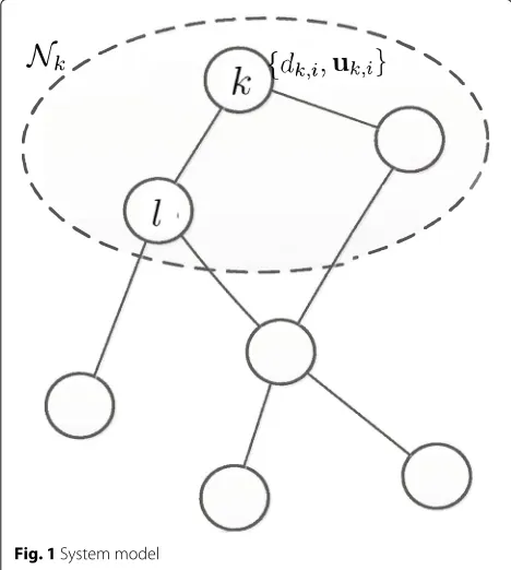
Let us consider a sensor network consisting ofN sensor nodes which are spatially distributed over a geographical area. The set of nodes connected to nodekincluding itself are called the neighbor nodes of nodek, denoted byNk. The number of the nodes linked to nodekis the degree ofk, denoted bynk. The system model for the distributed

estimation over sensor networks is presented in Fig. 1. At each time instanti, each nodekhas access to complex valued time realizations{dk,i,uk,i},k = 1, 2,. . .,N, i =

1, 2,. . ., with dk,i a scalar measurement and uk,i aM×1

input vector. The relation between the measurementdk,i

and the input vectoruk,ican be characterized as

dk,i=u∗k,iwo+vk,i (1)

where wo is the unknown optimal weight vector of size M×1, andvk,iis zero-mean additive white Gaussian noise

with varianceσ_v2_,k. Particularly, we assume that the noise variance has been determined in advance somehow. We also assume that the noise samplesvk,i, k = 1, 2,. . .,N, i = 1, 2,. . ., are independent of each other as well as the input vectorsuk,i. We aim to estimate the unknown

opti-mal weight vector wo in a distributed manner. That is, each sensor node k obtains a local estimate wk,i of size M×1 to approach the optimal weight vectorwoas much as possible. To this end, each nodeknot only uses its local measurementdk,iand input vectoruk,ibut also cooperates

with its closest neighbors for updating its local estimate wk,i. Specifically, by cooperation, each nodekhas access

to its neighbors’ data{dl,i,ul,i}and estimateswl,i at each

Fig. 1System model

time instantiwherel∈Nk, and then, each nodekfuses all the available information to update its local estimateψk,i.

Let us first introduce some vectors and matrices. At each time instanti, by collecting all nodes’ measurements into vectoryi, noise samples into vectorvi(both of length N), and input vectors into the matrixHiof sizeN×M, we

obtain

yi=col{d1,i. . .dN,i} Hi=col{u∗1,i. . .u∗N,i} vi=col{v1,i. . .vN,i}.

(2)

Following this, we define the covariance matrix of the noise vectorvias

Rv=E[viv∗i]=diag

σ2

v,1,σv2,2,. . .,σv2,N

. (3)

Next, we stackyi,viandHifrom time instant 0 to time

instantiinto matrices respectively, which are given by

Yi=col{yi. . .y0}

Hi=col{Hi. . .H0}

Vi=col{vi. . .v0}.

(4)

Besides, we defineRv,i=E[ViVi∗].

2.2 Brief review of diffusion-based DRLS algorithm

In this part, we give a brief introduction to the diffusion-based DRLS algorithm [6, 7].

For the diffusion-based DRLS algorithm, the local opti-mization problem to estimate the optimal weight vector woat each nodekcan be formulated as follows:

ψk,i=arg min_w

w2_i+ Yi−Hiw2_Wk,i

(5)

Note that the notation a2 = a∗a represents the weighted vector norm of any positive definite Hermitian matrix. Besides, the matrixiis given byi= λi+1

where 0 λ < 1 representing the forgetting factor and

= δ−1_I

M withδ > 0. Furthermore, the matrixWk,i

can be expressed asWk,i = R−v,i1idiag{Ck,Ck,. . .,Ck},

wherei = diag{IN,λIN,. . .,λiIN}andCk is a diagonal

matrix. It is worth noting that the main diagonal elements of the matrixCkis composed of thekth column of matrix C. Particularly, the matrixCis the adaptation matrix for the diffusion-based DRLS algorithm and satisfiesIT_C=I

The optimization problem (5) can be rewritten as

The closed-form solution to (6) is given by [6, 7]

ψk,i=Pk,iH∗iWk,iYi (7)

However, the closed-form solution in (7) is obtained via calculating the inversion of matrices, which requires large computation. Instead, the diffusion-based DRLS algo-rithm provides a recursive approach to solve (6), which can be implemented by the following two steps.

Step1: Let us take the updates at time instantifor exam-ple. Note that we denote the iteration number at time instantias the superscript(·)l_{withl=0 representing the}

initial value. At the very start, we initialize the intermedi-ate local estimintermedi-ateψ_k,iand the inverse matrixPk,ifor each

nodekby utilizing the updated results from time instant i−1, that is

ψ0

k,i=wk,i−1 P0_k,i=λ−1Pk,i−1

(9)

Then, for each nodek, its data is updated incrementally among its neighbors, which is given by

ψl

where the left arrow denotes the operation of assignment. Finally, each nodekobtains its ultimate intermediate local estimateψ_k,iwhich can be expressed as

ψk,i ←− ψ|kN,ik| (12)

Step2: Each nodekcombines the ultimate intermediate local estimate of its own, i.e.,ψ_k,i, obtained in step 1 with that of its neighbors, i.e.,ψ_l,i,l ∈ Nk by performing the following diffusion to obtain the local estimatewk,i:

wk,i= N

l=1

Al,kψl,i (13)

where Al,k denotes the (l,k)thelement of the matrixA.

Particularly, the matrixAis the combination matrix for

the diffusion-based DRLS algorithm and is chosen such thatITA=I[6].

Note that the steps (9)–(13) constitute the diffusion-based DRLS algorithm [6, 7].

3 Low-complexity variable forgetting factor mechanisms

In this section, we introduce the LTVFF mechanism and the LCTVFF mechanism that are employed by our proposed algorithms. Particularly, the analyses for the variable forgetting factor in terms of the steady-state properties of the first-order statistics are presented, and the LTVFF-DRLS algorithm that employs the LTVFF mechanism as well as the LCTVFF-DRLS algorithm that applies the LCTVFF mechanism are proposed. In the last part of this section, we analyze the computational com-plexity for these two VFF mechanisms as well as the proposed algorithms.

3.1 LTVFF mechanism

Motivated by the VSS mechanism [13, 14] for the diffusion LMS algorithm, the low-complexity VFF mechanisms are designed such that smaller forgetting factors are employed when the estimation errors are large in order to obtain a faster convergence speed, whereas the forgetting fac-tor increases when the estimation errors become small so as to yield better steady-state performance. Based on the above idea, an effective rule to adapt the forgetting factor can be formulated as

λk(i)=[ 1−ζk(i)]λ_λ+₋ (14)

where the quantityζk(i)is related to the estimation errors

and varies in an inverse way to the forgetting factor, which is referred to as the adaptation component. The operator [·]λ_λ+₋denotes the truncation of the forgetting factor to the limits of the range [λ+,λ−].

For the LTVFF mechanism, the adaptation component is given by

ζk(i)=αζk(i−1)+β|ek(i)|2 (15)

with parameters 0< α <1 andβ >0. Besides,αis cho-sen close to 1 andβis set to be a small value. The quantity ek(i)denotes the priori estimation error [19] of each node

for the DRLS algorithm, which can be expressed as ek(i)=dk,i−u∗k,iwk,i−1. (16) That is to say, in the LTVFF mechanism, the adapta-tion component is updated based on the instantaneous estimation error.

large estimation errors will cause an increase in the adap-tation componentζk(i), which yields a smaller forgetting

factor and provides a faster tracking speed. Conversely, small estimation errors will lead to the decrease of the adaptation componentζk(i), and thus, the forgetting

fac-tor λk(i) will be increased to yield smaller steady-state

misadjustment.

Next, we study the steady-state statistical properties of the adaptation componentζk(i)and the forgetting factor λk(i). Based on (15), it is reasonable to assume thatζk(i)

andζk(i−1)are approximately equivalent wheni→ ∞.

By taking expectations on both sides of (15) and lettingi goes to infinity, we can obtainE[ζk(∞)]

define the weight error vector for nodekas

where the termE

uT_k,iwk,i−1 2

denotes the excess error. Since it is sufficiently small when i → ∞ compared with the variance of noise, it can be neglected. As a consequence, the following approximation holds

E|ek(∞)|2

≈εmin (20)

whereεmindenotes the minimum mean-square error and can be expressed as

εmin=E

Subsequently, by substituting (20) into (17), we can approximately write

E[ζk(∞)]≈ β

1−αεmin. (22)

According to (14), we can deduce

E[λk(∞)]=1−E[ζk(∞)] . (23)

By substituting (22) into (23), we can obtain the first-order statistics of the forgetting factor for the LTVFF mechanism:

E[λ_k(∞)]=1− β

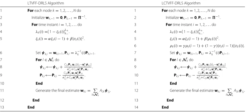
1−αεmin. (24) By applying the LTVFF mechanism to the diffusion-based DRLS algorithm, we propose the LTVFF-DRLS algorithm, which is exhibited in the left column of Table 1.

3.2 LCTVFF mechanism

For the LCTVFF mechanism, the forgetting factor can be calculated through (14) while the adaptation compo-nent ζk(i) can be adjusted according to an alternative

rule, that is, the time-averaged estimation of the correla-tion of two consecutive estimacorrela-tion errors is employed to the updating equation of the adaptation componentζk(i).

Therefore, the rule to update the adaptation component can be described as

ζk(i)=αζk(i−1)+β|ρk(i)|2 (25)

where 0< α <1 andβ >0. Particularly,αis set close to 1 andβis chosen to be slightly larger than 0. The quantity ρk(i)denotes the time-averaged estimation of the

correla-tion of two consecutive estimacorrela-tion errors, which is defined by

ρk(i)=γρk(i−1)+(1−γ )|ek(i−1)||ek(i)| (26)

where 0< γ <1 andγ is slightly smaller than 1. Note that the LCTVFF mechanism is given by (14), (25), and (26).

Next, we consider the steady-state statistical properties ofρk(i),ζk(i), andλk(i)for the LCTVFF mechanism. As

we will see in simulation results, the proposed algorithm converges to the steady-state in numerous iterations, and thus, the values ofρk(i− 1) and ρk(i) can be assumed

to be approximately equivalent, respectively, when i is large enough. Thus, we can obtainE[|ek(i−1)||ek(i)|]≈ E[|ek(i)|2] andρk(i−1) ≈ ρk(i)wheni → ∞. Then, by

taking expectations on both sides of (26) and lettingigo to infinity, we can obtain the first-order statistical properties ofρk(i):

E[ρk(∞)]≈εmin. (27)

To study the second-order statistical properties ofρk(i),

we consider the square of (26), which is given by ρ2

pared with other terms in (29), it can be neglected. Therefore, we can obtain

ρ2

k(i)≈γ2ρk2(i−1)+2γ (1−γ )ρk(i−1)|ek(i)|2. (30)

According to (16) and (26), the quantities ofρk(i−1)and |ek(i)|2can be considered uncorrelated at steady state, that

is to say,E[ρk(i−1)|ek(i)|2]≈E[ρk(i−1)]E[|ek(i)|2]. Note

Table 1LTVFF-DRLS and LCTVFF-DRLS algorithms

LTVFF-DRLS Algorithm LCTVFF-DRLS Algorithm

1 Foreach nodek=1, 2,. . .,Ndo 1 Foreach nodek=1, 2,. . .,Ndo 2 Initializewk,−1=0,Pk,−1=−1. 2 Initializewk,−1=0,Pk,−1=−1.

3 Fortime instanti=1, 2,. . .do 3 Fortime instanti=1, 2,. . .do 4 λk(i)=[ 1−ζk(i)]λλ+−. 4 λk(i)=[ 1−ζk(i)]

λ+

λ−.

5 ζk(i)=αζk(i−1)+β|ek(i)|2. 5 ζk(i)=αζk(i−1)+β|ρk(i)|2.

6 _ρk(i)=γρk(i−1)+(1−γ )|ek(i−1)||ek(i)|.

6 Set_ψk,i=wk,i−1,Pk,i=λ−_k1(i)Pk,i−1. 7 Setψk,i=wk,i−1,Pk,i=λ−_k1(i)Pk,i−1.

7 Forl_∈Nkdo 8 Forl∈Nkdo

8 _{ψk,i←−ψk,i+}Cl,kPk,iul,i[dl,i−u∗l,iψk,i] σ2

v,l+Cl,ku∗l,iPk,iul,i . 9 ψk,i←−ψk,i+

Cl,kPk,iul,i[dl,i−u∗l,iψk,i] σ2

v,l+Cl,ku∗l,iPk,iul,i .

9 Pk,i←−Pk,i−

Cl,kPk,iul,iu∗l,iPk,i σ2

v,l+Cl,ku∗l,iPk,iul,i. 10 Pk,i←−Pk,i−

Cl,kPk,iul,iu∗l,iPk,i σ2

v,l+Cl,ku∗l,iPk,iul,i.

10 End 11 End

11 Generate the final estimatewk,i=

l∈NkAl,kψl,i. 12 Generate the final estimatewk,i=

l∈NkAl,kψl,i.

12 End 13 End

13 End 14 End

Then, by taking expectations on both sides of (30), we can obtain the following result:

Eρ2_k(∞)= 2γ

1+γE[ρk(∞)]E

|ek(∞)|2

. (31)

Substituting (20) and (27) into (31) results in

Eρ2_k(∞)≈ 2γ 1+γε

2

min. (32) To calculate the first-order statistics of the adaptation component ζk(i), we take expectations on both sides of

(25) and letigoes to infinity, as a result, we obtain

E[ζk(∞)]= β

1−αE[ρ 2

k(∞)] . (33)

Substituting (32) into (33) leads to

E[ζk(∞)]=

2γβ (1+γ )(1−α)ε

2

min. (34) Consequently, we have the first-order steady-state statistics of the forgetting factor for the LCTVFF mecha-nism as follows:

E[λk(∞)]=1−

2γβ (1+γ )(1−α)ε

2

min. (35) By employing the LCTVFF mechanism to the diffusion-based DRLS algorithm, we propose the LCTVFF-DRLS algorithm, which is presented in the right column of Table 1.

3.3 Computational complexity

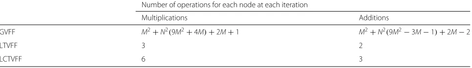
In this part, we study the computational complexity of the proposed LTVFF and LCTVFF mechanisms in compar-ison with the GVFF mechanism. Generally, we evaluate the number of arithmetic operations in terms of complex

additions and multiplications for each node at each iter-ation. The results have been shown in Tables 2 and 3. From Table 3, the additional computational complexity of the proposed LTVFF and LCTVFF mechanisms is evalu-ated by fixed small values for each node at each iteration. However, for the GVFF mechanism, the additional com-putational complexity increases with the size of the sensor network for each node at each iteration. The result in Table 3 clearly reveals that the proposed LTVFF and LCTVFF mechanisms greatly reduce computational cost when compared to the GVFF mechanism.

4 Performance analysis

In this section, we carry out the analyses in terms of mean and mean square error performance for the proposed LTVFF-DRLS and LCTVFF-DRLS algorithms. In partic-ular, we derive mathematical expressions to describe the steady-state behavior based on MSD and EMSE. In addi-tion, we also perform transient analysis in a specialized case for the proposed algorithms in the last part of this section. To proceed with the analysis, we first introduce several assumptions, which have been widely adopted in the analysis for the RLS-type algorithms and have been verified by simulations [7, 27].

Assumption 1To facilitate analytical studies, we assume that all the input vectorsuk,i,∀k,i are independent of each other and the correlation matrix of the input vector uk,iis invariant over time, which is defined as

E[uk,iuk∗,i]Ruk. (36)

Table 2Computational complexity of the DRLS algorithm

Number of operations for each node at each iteration

Multiplications Additions

DRLS (fixed forgetting factor) M2_+N2_(4M2_{+5M+1)+M 4N}2_M2_+M−1

exists a positive number Ni, when i > Ni, for which we have that the forgetting factorλk(i)varies slowly around its mean value, that is

E{λk(Ni)}E{λk(Ni+1)}. . .E{λk(i)}E{λk(∞)}.

(37)

For the RLS-type algorithms with the fixed forget-ting factor, we have the ergodicity assumption for Pk,i

[6, 7, 27], that is, the time average of a sequence of ran-dom variables can be replaced by its expected value so as to make the analysis for the performance of these algo-rithms tractable. Similarly, for the RLS-type algoalgo-rithms with variable forgetting factors, we still have the ergodicity assumption:

Assumption 3We assume that there exists a number Ni > 0, when i > Ni, for which we can replaceP−_k,i1by its expected value E

P−_k,1_i

, which can be represented as

lim

can be calculated through

lim

The derivation is presented in Appendix B. Since lim Moreover, based on the ergodicity assumption, it is also common in the analysis of the performance of the RLS-type algorithms to replace the random matrixPk,ibyPkwhen i is large enough.

4.1 Mean performance

In light of (1) and (13), the following relation holds [7] after the incremental update ofψ_l,iis complete:

P−_l,i1ψ_l,i=λl(i)P−l,i1−1wl,i−1+

By substituting (1) and (18) into (40), we obtain the following equation: Next, let us define the intermediate weight error vector

ψk,ifor nodekas

ψk,i=ψk,i−wo. (42)

Substituting (42) into (41) results in the following result:

enough (cf. Assumption 3), and thus, it is reasonable to assume thatPk,i converges asi → ∞. Therefore, we can

approximately have

Pk,i≈E[Pk,i] . (45)

Besides, in view of Assumption 3 and the Eq. (39), we can obtain By combining (45) and (46), we have the following approximation:

Table 3Additional computational complexity of the analyzed VFF mechanisms

Number of operations for each node at each iteration

Multiplications Additions

GVFF M2_+N2_(9M2_{+4M)+2M+1 M}2_+N2_(9M2_{−3M−1)+2M−2}

LTVFF 3 2

Then, substituting (47) into (44) yields the following result wheniis sufficiently large:

wk,i= Following this, two global matricesWiandP are built

in the following form in order to collect the weight error vectorswk,i,k=1,· · ·,Nand matricesPk,k =1,· · ·,N,

respectively:

Wi=row{w1,i,w2,i,. . .,wN,i}

P=row{P1,P2,. . .,PN}. (49)

In addition, we introduce a global diagonal matrixD(i) to collect the forgetting factors of all nodes at time instant i, which is given by To separate the noise vectors, we can rewrite (51) as

Gi=diag where ⊗ denotes the Kronecker product of two matri-ces [28]. Subsequently, we express (48) in a more compact way, which leads to the following updating equation for the global matrixWi:

Wi=Wi−1iA+PGiA. (53)

In order to simplify the notationiA, we denote it as F(i), and thus, we can rewrite (53) as

Wi=Wi−1F(i)+PGiA. (54)

In order to facilitate analysis, we assume that Wi−1 and F(i) can be considered uncorrelated, that is, E[Wi−1F(i)]≈ E[Wi−1]E[F(i)]. As we will see in simu-lation results, this assumption works well for theoretical analysis, which matches numerical results perfectly. By taking expectations on both sides of (54), we obtain the following result:

E[Wi]=E[Wi−1]E[F(i)]+PE[Gi]A. (55)

Recall (52), since the noise samplesvihave zero mean, E[Gi] equals to zero; therefore, we can obtain

E[Wi]=E[Wi−1]E[F(i)] . (56)

Following this, we assume that there exists a number Ni >0 and iterate (56) starting from the time instantito Ni, as a result, we obtain

have the following relation for each element inF(i):

Fm,n(i)=λm(i)Am,n(i),∀m,n∈ {1, 2,· · ·,N} (58)

where the subscriptm,nrepresents the(m,n)-th element in the matrix. Given that the elements ofAare all between 0 and 1 and each element in the diagonal matrixidoes

not exceed the upper bound λ+, which is smaller than unity, we have

Fm,n(i)=λm(i)Am,n(i) < λ+Am,n(i) <1,∀m,n∈ {1, 2,· · ·,N}

(59)

Each element in the product

i

are bounded in absolute value by some finite constant, therefore, all the elements ofE[Wi] converge to zero when i → ∞. As a result, we can conclude that the proposed LTVFF-DRLS and LCTVFF-DRLS algorithms converge asymptotically wheni→ ∞.

4.2 Mean-square error and deviation performances

In this part, we perform analyses for the proposed LTVFF-DRLS and LCTVFF-LTVFF-DRLS algorithms based on mean square performance and derive expressions for the steady-state MSD and EMSE, which are defined as

MSDss_k = lim

We start with (54) and then operate recursively from time instantNi, which yields

where ek is a column vector of lengthN with unity for

the kth element and zero for the others. Next, we write the Euclidean norm of the weight error vectorwk,i, that is, wk,i2, or equivalently,Tr{wk,iw∗_k,i}.

Since the elements ofF(i)are all bounded by zero and one,

i

j=Ni+1

F(j)vanishes wheni→ ∞, which leads to the

expectation of the first term becoming zero. Moreover, seeing that the cross terms incorporate the zero-mean vectors vi, their expectations also become zero. As a

result, we have the following expression:

Ewk,i2

which can be rewritten as

Ewk,i2

For simplicity, we have the following notation:

Jt,l(i)=A

According to the properties of the Kronecker product, we have the following equality:

(A⊗B)(C⊗D)=AC⊗BD. (66)

Therefore,(IN⊗vt)Jt,l(i)

)

IN⊗v∗_l

*

can be expressed as

(IN⊗vt)Jt,l(i) ance matrix of noiseRvcan be considered uncorrelated.

Then, by taking expectations on both sides of (67), we have the following results: substituting (68) into (64), we can obtain

Ewk,i2

have the following expression:

Ewk,i2

By taking expectations on both sides of (71), we obtain the following equality:

Substituting (65) and (72) into (70) yields the following result:

In view of Assumption 2, we can verify that there exists a numberNi>0, wheni>Ni, for whichF(i)satisfies

E[F(Ni)]E[F(Ni+1)]. . .E[F(i)]E[F(∞)] .

(74)

Therefore, we replaceE[F(i)] withE[F(∞)] wheni > Niand then reformulate (73) as

Subsequently, we replacei−twithtin (75) and then let igoes to infinity. As a result, we can obtain the expression of the steady-state MSD for nodek:

MSDss_k = lim

Next, we calculate the steady-state EMSE for node k. According to (60), the EMSE for nodekcan be expressed as follows (76) into (77), we can obtain the expression of the steady-state EMSE for nodek:

Expressions (76) and (78) describe the steady-state behavior of the proposed LTVFF-DRLS and LCTVFF-DRLS algorithms. By comparing the expressions (76) and (78) with the analytical results in [7], it is clear that the fixed matrixλ2Ain the expressions for the conventional DRLS algorithms has been replaced by the matrix F(i) in the expressions (76) and (78), which is weighted by the matrix i. Sincei varies from one iteration to the

next,F(i)varies for each iteration as well, which improves the tracking performance of the resulting algorithms. Fur-thermore, since all the elements inF(i) are bounded by zero and unity, the values of the steady-state MSD and EMSE given by (76) and (78) are both very small values wheniis large enough. Thus, we can verify that the pro-posed LTVFF-DRLS and LCTVFF-DRLS algorithms both converge in the mean-square sense.

4.3 Transient analysis under spatial invariance assumption

In this subsection, we consider a specialized case that the noise variances and input vector covariance matri-ces are the same for all the sensor nodes, and provide

transient analysis for this specific case. Particularly, we assume spatial invariance:

In addition, to facilitate analysis, we assume that all elements of the adaptation matrixCare equal to _N1.

We study the transient analysis through focusing on the learning curve, which is obtained by depicting the squared priori estimation error, i.e.,E

|u∗_k,i(wk,i−wo)|2

[29, 30], as a function of the iteration numberi. We first rewrite this squared priori estimation error in a more compact form:

Then, we use the spatial invariance assumption to sim-ply (39) and (48). Particularly, by taking advantage of the assumption that the input vector covariance matrix is the same over all sensor nodes, we can derive the following expression from (39), wheniis large enough:

Pk,i≈E By substituting (82) into (48), we can arrive at

˜ where we use the column vector si to denote the

Note thati = diag{λi}. Then, we can write the

recur-sive equation of type (83) for all sensor nodes in a more compact form as follows:

˜

have the following global squared priori estimation error for all sensor nodes by using the last equality in (85):

E[ ˜Wi2Ru]=E[W˜

Kronecker product, i.e., (66), in the fourth and fifth equal-ities, and the fact that both quantities off(i)T_R

uf(i)and s∗_isi are scalar and they are independent to arrive at the

last equality. Particularly,E[s∗_isi] can be rewritten as E[s∗_isi]

where we use the spatial invariance assumption, i.e., viv∗i = diag{σv2,σv2,· · ·,σv2} = σv2IN and H∗iHi =

_N

m=1um,iu∗m,i=

_N

m=1Rum =NRu, to arrive at the third

and fourth equalities, respectively, and the symmetry of the input vector covariance matrix in the last equality. By plugging (87) back into (86), we have

E sents the vectorization of a matrix. Particularly, by using

the equality vec{ABC} =(CT⊗A)vec{B}, we can vector-This recursive equation is stable and convergent if E[Fi] is stable [31].

Particularly, the quantity Fi has a spectral radius

smaller than unity and thus is stable. This can be proved as follows: If we replace each element iniby its upper

boundλ+, then we haveFireplacced byλ2+A⊗A. Note thatAsatisfiesITA = I, and then, we can readily verify that each column ofA⊗Asums up to unity. Hence, the quantityλ2₊A⊗Ahas the spectral radiusλ2₊that is smaller than one. Given that each element inidoes not exceed λ+, the spectral radius ofFiis smaller thanλ2+and surely is smaller than unity. Therefore, for this specialized case, it can be verified theoretically that the proposed LTVFF-DRLS and LCTVFF-LTVFF-DRLS algorithms are convergent in terms of the learning curve and the convergence rate is related to the varying forgetting factors.

Also note that, since the convergence performance of the adaptive algorithms does not depend on the outside environment but rely on the network topology and the design of algorithms, the analytical results in this special-ized case also apply to the general case.

5 Simulation results

In this section, we present the simulation results for the proposed LTVFF-DRLS and LCTVFF-DRLS algorithms when applied in two applications, that is, distributed parameter estimation and distributed spectrum estima-tion over sensor networks.

5.1 Distributed parameter estimation

0 0.2 0.4 0.6 0.8 1 0

0.1 0.2 0.3 0.4 0.5 0.6 0.7 0.8 0.9 1

1

2 3

4

5

6 7

8

9 10

Fig. 2Network topology for the simulation results in Section 5.1

factor and the GVFF-DRLS algorithm. In addition, we also verify the effectiveness of the proposed analytical expressions in (76) and (78) based on simulations.

We assume that there are 10 nodes in the sensor net-work and the length of the unknown weight vector isM= 5. The input vectorsuk,i,k = 1, 2,. . .,N are assumed to

be Gaussian with zero means and variances

σ2

u,k

chosen randomly between 1 and 2 for each node. The Gaussian noise samplesvk,i,k = 1, 2,. . .,Nhave variances

σ2

v,k

that are chosen randomly between 0.1 and 0.2 for each node. We generate the measurements{dk,i}according to

(1). Simulation results are averaged over 100 experiments. The adaptation matrixC is governed by the Metropolis

rule, while the choice of the diffusion matrixAfollows the relative-degree rule [8]. The network topology used for the simulations is shown in Fig. 2.

5.1.1 Effects ofα,β, andγ

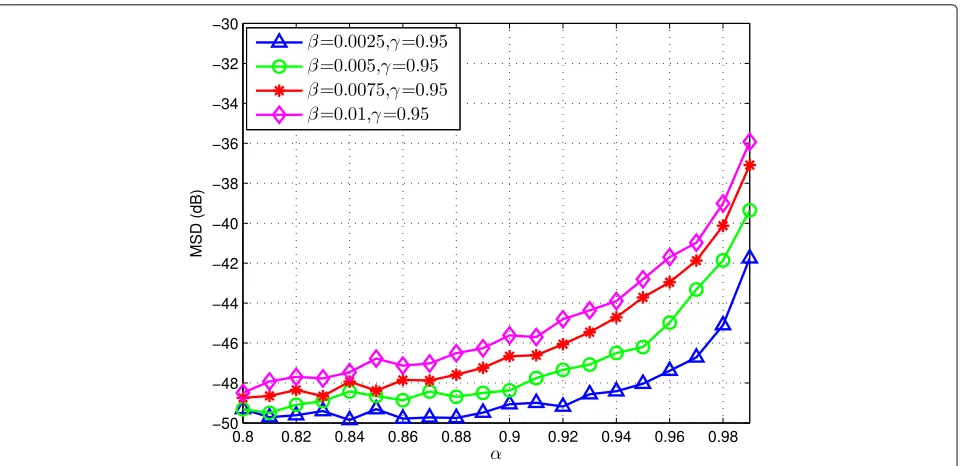
In this subsection, we study the effects of the parame-ters α, β, and γ on the performance of the proposed LTVFF and LCTVFF mechanisms. For the LTVFF mech-anism, we investigate the steady-state MSD values versus α for β = 0.0015, 0.002, 0.0025, 0.005. The simulation results are shown in Fig. 3. For the LCTVFF mecha-nism, we first depict the steady-state MSD values versus α forβ = 0.0025, 0.005, 0.0075, 0.01 in Fig. 4. Then, the effects of γ are illustrated in Fig. 5 by investigating the steady-state MSD values againstγ for different pairs ofα andβ.

As can be seen from Figs. 3 and 4 for both the LTVFF and LCTVFF mechanisms, the optimal choice of α and β is not unique. Specifically, different pairs of α and β can yield the same steady-state MSD value. For exam-ple, for the LTVFF mechanism, the pairsα = 0.91,β = 0.0015,α = 0.89,β = 0.002, andα = 0.87,β = 0.0025 provide almost the same steady-state MSD performance. For the LCTVFF mechanism, whenγ = 0.95, the pairs α = 0.93,β = 0.0025, α = 0.90,β = 0.005, α = 0.85,β =0.0075, andα=0.80,β =0.01 yield almost the same steady-state MSD value. In addition, it can also be observed that with the decreasing ofαandβ, the steady-state performance degrades. Furthermore, the result in Fig. 5 reveals that the steady-state MSD performance of the LCTVFF mechanism does not change so much asγ varies for different pairs ofαandβ.

Fig. 4Steady-state MSD versus_αfor different values of_βfor the LCTVFF mechanism when_γ=0.95

However, when we choose appropriate values for α, β, and γ, only considering the effects on the steady-state behaviors is not enough. This is because that the convergence speed is closely connected to the steady-state MSD values. That is to say, when the algorithm assumes a faster convergence speed, the steady-state error floor rises; if the convergence speed is controlled to be slower, the steady-state performance improves.

Figures 6 and 7 show the trade-off between conver-gence speed and steady-state performance by depicting learning curves against different values of α and β for LTVFF-DRLS and LCTVFF-DRLS algorithms, respec-tively. Therefore, we need to keep a good balance between the steady-state behaviors and the convergence speed in order to ensure good performance. In practical applica-tions, the optimized values of α, β, and γ should be

Fig. 6Learning curves against different values ofαandβfor LTVFF-DRLS algorithm

obtained through experiments and then stored for the future use.

5.1.2 MSD and EMSE performance

Figures 8 and 9 show the MSD curves against the num-ber of iterations for the LTVFF-DRLS and LCTVFF-DRLS algorithms with different initial values for the forgetting factor in comparison with the conventional DRLS algo-rithm and the GVFF-DRLS algoalgo-rithm, respectively. The parameters of the considered algorithms are listed in

Table 4. From the results, the LTVFF-DRLS algorithm converges to almost the same error floor in two scenar-ios where the variable forgetting factor is initialized to be small or large. This is also true for the LCTVFF-DRLS algorithm, which has lower error floor and faster conver-gence speed than the LTVFF-DRLS algorithm. However, as shown in Fig. 8, for the conventional DRLS algorithm, its convergence speed and steady-state error floor both have obvious changes when the fixed forgetting factors increases. Specifically, when the fixed forgetting factor is

200 400 600 800 1000 1200 1400 1600 1800 2000 −50

−45 −40 −35 −30 −25 −20 −15 −10

Number of Iterations

MSD (dB)

LTVFF−1 LCTVFF−1 LTVFF−2 LCTVFF−2 fixed−1 fixed−2

Fig. 8MSD performance against iterations for the proposed algorithms with different initial values for the forgetting factor compared with the DRLS algorithm with the fixed forgetting factor

small, the conventional DRLS algorithm converges faster but has a higher error floor than the LTVFF-DRLS algo-rithm; however, as the fixed forgetting factors increase, it converges to a lower error floor (not as good as the LTVFF-DRLS algorithm) but has slower convergence speed. Besides, from Fig. 9, the MSD performance of the proposed LTVFF-DRLS and LCTVF-DRLS algorithms are

less sensitive to the initial values for the forgetting fac-tor than that of the GVFF-DRLS algorithm. Therefore, by employing the LTVFF and LCTVFF mechanisms, the proposed algorithms can track the optimal performance regardless of the initial values for the forgetting factor and greatly reduce the difficulty in choosing the appropriate value for the forgetting factor.

200 400 600 800 1000 1200 1400 1600 1800 2000 −50

−45 −40 −35 −30 −25 −20 −15 −10

Number of Iterations

MSD (dB)

LTVFF−1 LCTVFF−1 LTVFF−2 LCTVFF−2 GVFF−1 GVFF−2

Table 4Optimized parameters for different algorithms considered in Figs. 8 and 9

LTVFF-1 α=0.91,β=0.0015

λ0=0.995,λ+=0.9998,λ₋=0.980 LTVFF-2 α=0.91,β=0.0015

λ0=0.950,λ+=0.9998,λ−=0.950

LCTVFF-1 α=0.95,β=0.005,γ =0.95 λ0=0.995,λ+=0.9998, ,λ−=0.950 LCTVFF-2 _α=0.95,_β=0.005,_{γ =}0.95

λ0=0.950,λ+=0.9998, ,_λ−=0.950 GVFF-1 _λ0=0.995,μ=0.005,λ+=0.9998,_λ−=0.990 GVFF-2 λ0=0.950,μ=0.005,λ+=0.9998,λ₋=0.950

Fixed-1 λ=0.998

Fixed-2 λ=0.995

Fixed-3 λ=0.950

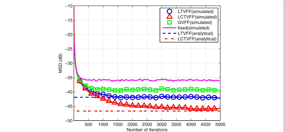
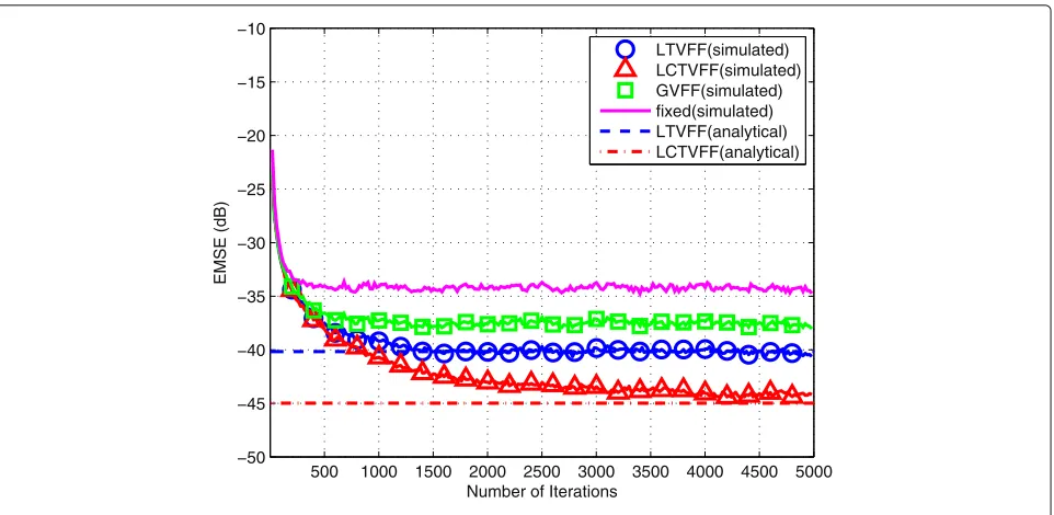
In Figs. 10, 11, 12, and 13, we evaluate the performance of the proposed LTVFF-DRLS and LCTVFF-DRLS algo-rithms based on MSD and EMSE behaviors in comparison with that of the conventional DRLS with the fixed forget-ting factor and the GVFF-DRLS algorithms. Specifically, the MSD and EMSE curves against the number of itera-tions for the analyzed algorithms are depicted in Figs. 10 and 11, respectively, while the steady-state MSD and EMSE values for each node are shown in Figs. 12 and 13, respectively. As can be seen from these results, both the LTVFF-DRLS and LCTVFF-DRLS algorithms converge

after a number of iterations and achieve lower steady-state MSD and EMSE values compared to the DRLS algo-rithm with the fixed forgetting factor and the GVFF-DRLS algorithm. Besides, we also depict the analytical results which are calculated through expressions (76) and (78) in Figs 10, 11, 12, and 13. From these results, it is clear that analytical expressions corroborate the simulated results very well. The parameters of the considered algorithms are shown in Table 5, which are tuned through experi-ments by referring to the investigation in Section 5.1.1.

In Fig. 14, we test the performance of different algo-rithms considered in a non-stationary environment. Specifically, in order to simulate the non-stationary envi-ronment, we consider the scenario where the topology of the sensor network varies over time, that is, the total number of sensor nodes is set to 40 at the start, and then, we switch off half of the nodes after 100 iter-ations and another 10 nodes after 800 iteriter-ations. The MSD curves against the number of iterations for the pro-posed algorithms in comparison with the conventional DRLS algorithm with the fixed forgetting factor and the GVFF-DRLS algorithm in the non-stationary environ-ment are depicted in Fig. 14. As can be observed, the switching off of some sensor nodes results in the degra-dation of the performance for all the algorithms. How-ever, the proposed LTVFF-DRLS and LCTVFF-DRLS algorithms still outperform the other two existing algo-rithms in MSD performance. Besides, they exhibit better tracking properties by showing smaller and smoother variations in the MSD curves at the time of switching sensor nodes.

500 1000 1500 2000 2500 3000 3500 4000 4500 5000 −50

−45 −40 −35 −30 −25 −20 −15 −10

Number of Iterations

MSD (dB)

LTVFF(simulated) LCTVFF(simulated) GVFF(simulated) fixed(simulated) LTVFF(analytical) LCTVFF(analytical)

500 1000 1500 2000 2500 3000 3500 4000 4500 5000 −50

−45 −40 −35 −30 −25 −20 −15 −10

Number of Iterations

EMSE (dB)

LTVFF(simulated) LCTVFF(simulated) GVFF(simulated) fixed(simulated) LTVFF(analytical) LCTVFF(analytical)

Fig. 11EMSE curve against number of iterations for the proposed and existing algorithms

Next, we elaborate the numerical stability of the proposed LTVFF-DRLS and LCTVFF-DRLS algorithms. Through tuning the parametersα,β,γ,λ+,λ+to different values, the proposed LTVFF-DRLS and LCTVFF-DRLS algorithms can have different convergence speed and steady-state performance, but their MSD and EMSE curves always decrease to the steady-state. Indeed, after a number of experiments, we have not encountered the case where they diverge. Hence, the proposed LTVFF and

LCTVFF mechanisms do not make the numerical stabil-ity of the DRLS algorithm worse. Besides, the simulation results in Fig. 14 show that, after switching some nodes in the network, the proposed LTVFF-DRLS and LCTVFF-DRLS algorithms still achieve superior performance to the conventional DRLS algorithm, and they exhibit smoother MSD curves at the time of switching nodes, especially the LCTVFF-DRLS algorithm. This further verifies that the proposed algorithms improve instead of impair the

1 2 3 4 5 6 7 8 9 10

−50 −45 −40 −35 −30 −25 −20 −15 −10

Node

Steady−State MSD (dB)

LTVFF (simulated) LCTVFF (simulated) fixed (simulated) GVFF (simulated) LTVFF (analytical) LCTVFF (analytical)

1 2 3 4 5 6 7 8 9 10 −50

−45 −40 −35 −30 −25 −20 −15 −10

Node

Steady−State EMSE (dB)

LTVFF (simulated) LCTVFF (simulated) fixed (simulated) GVFF (simulated) LTVFF (analytical) LCTVFF (analytical)

Fig. 13Steady-state EMSE value versus node for the proposed and existing algorithms

numerical stability of the DRLS algorithm by keeping better tracking of the variations.

5.2 Distributed spectrum estimation

In this part, we extend the proposed LTVFF-DRLS and LCTVFF-DRLS algorithms to the application of dis-tributed spectrum estimation, for which we focus on estimating the parameter w0 that is relevant to the unknown spectrum of a transmitted signals. First of all, we characterize the system model of distributed spectrum estimation.

We denote the power spectral density (PSD) of the unknown spectrum of the transmitted signalsby s(f),

which can be well approximated by the following basis expansion model [32] withNbsufficiently large:

s(f)= Nb

m=1

bm(f)w0m=bT0(f)w0 (91)

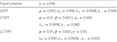
Table 5Optimized parameters for different algorithms considered in Figs. 10, 11, 12, and 13

Fixed scheme λ=0.990

GVFF μ=0.005,λ0=0.990,λ+=0.9998,λ₋=0.990 LTVFF α=0.91,β=0.0015,λ0=0.990

λ+=0.9998,λ₋=0.980 LCTVFF α=0.95,β=0.005,γ =0.95

λ0=0.990,λ+=0.9998, ,λ₋=0.950

where b0(f) = col{b1(f),b2(f),. . .,bNb(f)}is the vector

of basis functions [33, 34],w0=col{w01,w02,. . .,w0Nb}is

the expansion parameter to be estimated and represents the power that transmits the signalsover each basis, and Nbis the number of basis functions.

We assumeHk(f,i)to be the channel transfer function

between the source emitting the signalsand the receiver nodek at time instant i. Based on (91), the PSD of the signal received by nodekcan be represented as

r(f)= |Hk(f,i)|2s(f)+σ_r2_,k

= Nb

m=1

|Hk(f,i)|2bm(f)w0m+σr2,k

=bT_k,i(f)w0+σ_r2_,k

(92)

where bk,i(f) =

|H_k(f,i)|2_b

m(f)

Nb

m=1 ∈ RNb and σ 2

r,k

denotes the receiver noise power at nodek.

At each time instant i, by observing the received PSD described in (92) overNcfrequency samplesfj = fmin : (fmax−fmin)/Nc : fmax, forj = 1, 2,. . .,Nc, each nodek

takes measurements according to the following model:

dj_k,i=bT_k,i(fj)w0+σ_r2_,k+vj_k,i (93)

wherevj_k,idenotes the sampling noise at frequencyfjwith

zero mean and variance σ_n2_,j. The receiver noise power σ2

200 400 600 800 1000 1200 1400 1600 1800 2000 −50

−45 −40 −35 −30 −25 −20 −15

−10

Number of Iterations

MSD (dB)

LTVFF LCTVFF GVFF fixed

Fig. 14MSD performance against number of iterations for the proposed and existing algorithms in a nonstationary environment

and then subtracted from (93) [35, 36]. Therefore, we can obtain

d_kj_,i=bT_k,i(fj)w0+vj_k,i. (94)

By collecting the measurements over Nc frequencies

into a column vectordk,i, we obtain the following system

model of distributed spectrum estimation:

dk,i=Bk,iw0+vk,i. (95)

where dk,i =

df_kj_,i

Nc

j=1 ∈ R

Nc_{, B} k,i =

bT_k,i(fj)

Nc

j=1 ∈ RNc×Nb_{, withN}

c>Nb, andvk,i=

vj_k,i

Nc

j=1∈R

Nc_.

Next, we carry out simulations to show the performance of the proposed algorithms when applied to distributed spectrum estimation. We consider a sensor network com-posed of N = 20 nodes in order to estimate the unknown expansion parameterw0. We useNb=50

non-overlapping rectangular basis functions with amplitude

0 50 100 150 200 250 300 −45

−40 −35 −30 −25 −20 −15

Number of iterations

MSD( dB)

LTVFF LCTVFF GVFF fixed

Table 6Simulation time of running different algorithms in Figs. 15 and 16

Simulation time (seconds)

LTVFF 61.11

LCTVF 66.35

GVFF 176

fixed 73

equal to one to approximate the PSD of the unknown spectrum. The nodes can scanNc=100 frequencies over

the frequency axis, which is normalized between 0 and 1. In particular, we assume that only 8 entries ofw0are non-zero, which implies that the unknown spectrum is transmitted over 8 basis functions. Thus, the sparsity ratio equals to 8/50. We set the power transmitted over each basis function to be 0.7 and the variance of the sampling noise to be 0.004.

In Fig. 15, we compare the performance of different algorithms for the distributed spectrum estimation in terms of MSD. As can be depicted, the proposed LTVFF-DRLS and LCTVFF-LTVFF-DRLS algorithms still outperform the conventional DRLS algorithm in steady-state perfor-mance. By tuning parameters, the GVFF-DRLS algorithm can achieve similar performance to the proposed algo-rithms in the convergence speed and steady-state MSD values but at huge computational cost. We have listed the simulation time of running each algorithm for 600 iterations and 1 Monte Carlo experiment in Table 6.

As can be observed, the simulation time of running the GVFF-DRLS algorithm is almost 3 times of that for run-ning the other algorithms. In Fig. 16, we take node 1 as an example to investigate the performance of different algorithms in estimating the true PSD. From the results, although different algorithms obtain similar estimates of the true PSD, the proposed LCTVFF-DRLS algorithm obviously leads to smaller side lobes in the PSD curve than the other three.

6 Conclusions

In this paper, we have proposed two low-complexity VFF-DRLS algorithms for distributed estimation includ-ing the LTVFF-DRLS and LCTVFF-DRLS algorithms. For the LTVFF-DRLS algorithm, the forgetting factor is adjusted by the time-averaged cost function, while for the LCTVFF-DRLS algorithm, the forgetting factor is adjusted by the time-averaged of the correlation of two successive estimation errors. We also have investigated the computational complexity of the low-complexity VFF mechanisms as well as the proposed VFF-DRLS algo-rithms. In addition, we have carried out the convergence and steady-state analysis for the proposed algorithms. Moreover, we also have derived analytical expressions for the steady-state MSD and EMSE. The simulation results have shown the superiority of the proposed algorithms to the conventional DRLS and GVFF-DRLS algorithms in applications of distributed parameter estimation and distributed spectrum estimation and have verified the effectiveness of our proposed analytical expressions for the steady-state MSD and EMSE.

0 0.2 0.4 0.6 0.8 1

−40 −35 −30 −25 −20 −15 −10 −5 0

Frequency

PSD(dB)

LTVFF LCTVFF GVFF fixed true PSD

Appendices

A: Proof of the uncorrelation ofρk(i−1)and|ek(i)|2in the steady state

By multiplying both sides of (26) by |ek(i)|2 and taking

expectaitons, we have the following equation:

Eρk(i−1)|ek(i)|2

equivalent wheni→ ∞; therefore, we have the following results:

By recalling (27), we can obtain

Eρk(i−1)|ek(i)|2

uncorrelated in the steady state.

B: Proof of (39)

According to (8), we can obtain the following equation:

P−_k,1_i =

Therefore, (99) can be reformulate as

P−_k,1_i =λk(i)

Substituting (2) into (101) yields the following recursion:

P−_k,1_i =λk(i)P−_k,i1₋₁+

By employing the iterative Eq. (102), we can write

P−_k,i1= Recalling Assumption 1, we know that the correlation matrix of the input vector is invariant over time, as a result, the correlation matrixRul,i can be represented as Rul. Therefore, by taking expectations on both sides of

(103), we obtain the following result

E In view of Assumption 2, (104) can be approximately rewritten as whereξandχcan be expressed as follows, respectively:

and

Since ni is a finite positive number, ξ andχ are two

deterministic values. In addition, note thatλ_k(i)does not exceed its upper boundλ+, which is smaller than but close to unity. Therefore, we have 0 < E[λk(i)]< λ+ < 1,

and E[λk(i)]i−Ni+1< λi+−Ni+1. When i is large enough,

λi−Ni+1

+ approaches zero, and, of course, E[λk(i)]i−Ni+1

also approaches zero. As a result, the last term in (105) vanishes. Then, we obtain the following result:

lim

mechanism and in (35) for the LCTVFF mechanism, respectively. Hence, we obtain (39). Note that, by setting appropriate truncation bounds forλk(i), the steady-state

forgetting factor value will not be influenced by the trun-cation. Hence, the result (39) always holds true despite the truncation employed to the VFF mechanisms. Indeed, the truncation mechanism only plays a role during the process of converging. Once the algorithms reach the steady state, the values of the forgetting factor are not affected by the truncation mechanism any longer.

Funding

This work was supported in part by the National Natural Science Foundation of China under Grant 61471319, the Scientific Research Project of Zhejiang Provincial Education Department under Grant Y201122655, and the Fundamental Research Funds for the Central Universities.

Authors’ contributions

YC and RCdL proposed the original idea. LZ carried out the experiment. In addition, LZ and YC wrote the paper. CL and RCdL supervised and reviewed the manuscript. All authors read and approved the final manuscript.

Competing interests

The authors declare that they have no competing interests

Publisher’s Note

Springer Nature remains neutral with regard to jurisdictional claims in published maps and institutional affiliations.

Author details

1_{College of Information Science and Electronic Engineering, Zhejiang}

University, Hangzhou, People’s Republic of China.2_{CETUC-PUC-Rio, Rio de}

Janeiro, Brazil.

Received: 9 November 2016 Accepted: 6 July 2017

References

1. P Corke, T Wark, R Jurdak, W Hu, P Valencia, D Moore, Environmental wireless sensor networks. Proc. IEEE.98(11), 1903–1917 (2010)

2. JG Ko, C Lu, MB Srivastava, JA Stankovic, A Terzis, M Welsh, Wireless sensor networks for healthcare. Proc. IEEE.98(11), 1947–1960 (2010)

3. R Abdolee, B Champagne, AH Sayed, inProc. IEEE Statistical Signal Processing Workshop. Diffusion LMS for Source and Process Estimation in Sensor Networks (IEEE, Ann Arbor, 2012)

4. R Abdolee, B Champagne, AH Sayed, inProc. IEEE ICASSP. Diffusion LMS Localization and Tracking Algorithm for Wireless Cellular Networks (IEEE, Vancouver, 2013)

5. R Abdolee, B Champagne, AH Sayed, Diffusion adaptation over multi-agent networks with wireless link impairments. IEEE Trans. Mob. Comput.15(6), 1362–1376 (2016)

6. FS Cattiveli, CG Lopes, AH Sayed, inProc. IEEE Workshop Signal Process. Advances Wireless Commun. (SPAWC). A Diffusion RLS Scheme for Distributed Estimation over Adaptive Networks (IEEE, Helsinki, 2007), pp. 1–5

7. FS Cattiveli, CG Lopes, AH Sayed, Diffusion recursive least-squares for distributed estimation over adaptive networks. IEEE Trans. Signal Process.

56(5), 1865–1877 (2008)

8. FS Cattiveli, AH Sayed, Diffusion LMS strategies for distributed estimation. IEEE Trans. Signal Process.58(3), 1035–1048 (2010)

9. CG Lopes, AH Sayed, Diffusion least-mean squares over distributed networks: formulation and performance analysis. IEEE Trans. Signal Process.56(7), 3122–3136 (2008)

10. Y Liu, C Li, Z Zhang, Diffusion sparse least-mean squares over networks. IEEE Trans. Signal Process.60(8), 4480–4485 (2012)

11. S Xu, RC de Lamare, HV Poor, inProc. IEEE ICASSP. Adaptive link selection strategies for distributed estimation in diffusion wireless networks (IEEE, Vancouver, 2013)

12. S Xu, RC de Lamare, HV Poor, Distributed compressed estimation based on compressive sensing. IEEE Signal Process. Lett.22(9), 1311–1315 (2015) 13. MOB Saeed, A Zerguine, SA Zummo, A variable step-size strategy for

distributed estimation over adaptive networks. EURASIP J. Adv Signal Process.2013(1), 1–14 (2013)

14. H Lee, S Kim, J Lee, W Song, A variable step-size diffusion LMS algorithm for distributed estimation. IEEE Trans. Signal Process.63(7), 1808–1820 (2015)

15. Z Liu, Y Liu, C Li, Distributed sparse recursive least-squares over networks. IEEE Trans. Signal Process.62(6), 1386–1395 (2014)

16. S Huang, C Li, Distributed sparse total least-squares over networks. IEEE Trans. Signal Process.63(11), 2986–2998 (2015)

17. C Li, P Shen, Y Liu, Z Zhang, Diffusion information theoretic learning for distributed estimation over network. IEEE Trans. Signal Process.61(16), 4011–4024 (2013)

18. Z Liu, C Li, Y Liu, Distributed censored regression over networks. IEEE Trans. Signal Process.63(20), 5437–5449 (2015)

19. S Haykin,Adaptive Filter Theory, 4th edn. (Prentic-Hall, Englewood cliffs, 2000)

20. S Leung, CF So, Gradient-based variable forgetting factor RLS algorithm in time-varying environments. IEEE Trans. Signal Process.53(8), 3141–3150 (2005)

21. CF So, SH Leung, Variable forgetting factor RLS algorithm based on dynamic equation of gradient of mean square error. Electron. Lett.37(3), 202–203 (2011)

22. S Song, J Lim, S Baek, K Sung, Gauss Newton variable forgetting factor recursive least squares for time varying parameter tracking. Electron. Lett.

36(11), 988–990 (2000)

23. S Song, J Lim, SJ Baek, K Sung, Variable forgetting factor linear least squares algorithm for frequency selective fading channel estimation. IEEE Trans. Vehi. Techonol.51(3), 613–616 (2002)

24. F Albu, inProc. of ICARCV 2012. Improved Variable Forgetting Factor Recursive Least Square Algorithm (IEEE, Guangzhou, 2012) 25. Y Cai, RC de Lamare, M Zhao, J Zhong, Low-complexity variable

forgetting factor mechanisms for blind adaptive constrained constant modulus algorithms. IEEE Trans. Signal Process.60(8), 3988–4002 (2012) 26. L Qiu, Y Cai, M Zhao, Low-complexity variable forgetting factor

mechanisms for adaptive linearly constrained minimum variance beamforming algorithms. IET Signal Process.9(2), 154–165 (2015) 27. R Arablouei, K Dogancay, S Werner, Y Huang, Adaptive distributed

estimation based on recursive least-squares and partial diffusion. IET Signal Process.62(14), 1198–1208 (2014)

28. DS Tracy, RP Singh, A new matrix product and its applications in partitioned matrix differentiation. Statistica Neerlandica.51(3), 639–652 (2003)

29. H Shin, AH Sayed, inProc. IEEE ICASSP. Transient Behavior of Affine Projection Algorithms (IEEE, Hong Kong, 2003)