R E S E A R C H
Open Access
Accelerating the image processing by the
optimization strategy for deep learning
algorithm DBN
Changtian Ying
1,2, Zhen Huang
2and Changyan Ying
2*Abstract
In recent years, image processing especially for remote sensing technology has developed rapidly. In the field of remote sensing, the efficiency of processing remote sensing images has been a research hotspot in this field. However, the remote sensing data has some problems when processing by a distributed framework, such as Spark, and the key problems to improve execution efficiency are data skew and data reused. Therefore, in this paper, a parallel acceleration strategy based on a typical deep learning algorithm, deep belief network (DBN), is proposed to improve the execution efficiency of the DBN algorithm in Spark. First, the re-partition algorithm based on the tag set is proposed to the relief data skew problem. Second, the cache replacement algorithm on the basis of characteristics is proposed to automatic cache the frequently used resilient distributed dataset (RDD). By caching RDD, the re-computation time of frequently reused RDD is reduced, which lead to the decrease of total
computation time of the job. The numerical and analysis verify the effectiveness of the strategy.
Keywords:Deep learning, DBN, Acceleration strategy, Data skew, RDD cache
1 Introduction
With the improvement of observation ability in the field of big data [1–3] and the coexistence data of different imaging methods, wave bands, and resolution levels, re-mote sensing (RS) data has the characteristics of getting data in a short cycle, from a wide boundary and growing exponentially. In sharp contrast with remote sensing data acquisition ability, the processing ability of remote sensing information is relatively lower, and big data, small knowledge status has caused a certain degree of data disaster.
At present, with the combination of various fields and remote sensing technology becoming more and more close, the demand for using remote sensing images to
accurately distinguish geographical information is
highlighted. Many deep learning models are used in re-mote sensing image processing, such as Zhang et al. [4] made a technical tutorial on the state of the art for deep learning about remote sensing data, and Das and Ghosh
[5] presented a deep learning approach for spatiotempo-ral prediction of remote sensing data. Hinton et al. [6] gave deep neural networks for acoustic modeling in speech recognition. Badrinarayanan et al. [7] constructed a deep convolutional encoder-decoder architecture for image segmentation. Compared with traditional neural networks and support vector machines, the accuracy of recognition using convolutional neural networks was im-proved. Mou et al. [8] presented a convolutional neural network (CNN) extraction of visual features which is more suitable for image retrieval. From the above, it can be seen that the deep learning model shows a strong ability for learning and generalization of remote sensing data and can better facilitate remote sensing image clas-sification and identification of features. Deep belief
net-work (DBN) algorithm has high learning and
generalization ability for data and has achieved a lot of achievements in the field of image processing and net-work applications. For example, Dahl et al. [9] improved context-dependent pre-trained deep neural networks for
large vocabulary speech recognition. Chen et al. [10]
made spectral-spatial classification of hyperspectral data
based on deep belief network. Fischer and Igel [11]
* Correspondence:[email protected]
2School of Information Science and Engineering, Xinjiang University, Urumqi 830008, People’s Republic of China
Full list of author information is available at the end of the article
trained restricted Boltzmann machines. Tran et al. [12] proposed an approach to fault diagnosis of reciprocating compressor valves using deep belief networks.
However, the deep learning algorithm has high com-putational complexity and requires multiple iterations to make the parameters converge to an optimal value. This results in the low efficiency and time overhead of data classification by the deep learning algorithm. The exist-ing researches considered few about the data skew and
replacement during the task assignment on an
in-memory framework which leads to the increase of computation time.
In order to improve the efficiency of DBN, a parallel acceleration strategy for DBN (PA_DBN) is proposed, which includes re-partition algorithm and RDD (resilient distributed data) cache algorithm based on reused fre-quency and RDD size. Re-partition algorithm is used to solve the problem of data skew, and RDD cache algo-rithm is used to solve the problem of data reused. Then the strategy is verified effectiveness on the basis of re-mote sensing data processing.
2 Model definition and analysis 2.1 Basic model for DBN
The core architecture of the DBN algorithm is restricted Boltzmann machines (RBM). RBM simplifies the link be-tween the visual layer and a hidden layer of the Boltz-mann machine.
Definition 1Joint distribution function of RBM. Sup-pose there arem nodes in the visual layer, in which the ith node is represented byvi, and the hidden layer is
rep-resented by n nodes, where the jth node is represented
byhj. Assume the visual layer asv= (v1,v2⋯,vm) and the
resents the weight value between hidden nodejand
vis-ual node i, the bias value of visual layer node i denotes as ai, and the bias value of hidden node j denotes asbj.
When the parameters are determined, the joint distribu-tion funcdistribu-tion of RBM is defined as:
p vð ;hjθÞ ¼ 1
Zð Þθ expðð−E vðð ;hj Þθ ÞÞ ð2Þ
Zð Þ ¼θ X v;h
expðð−E vðð ;hj Þθ ÞÞ ð3Þ
Definition 2Softmax function. This function is a clas-sifier function, and since logical regression is a linear
regression model, it is often used to solve the classifica-tion problem. For the specific testing set {((x(1)),,y(2))),
whereθ is the parameter of the model, andkrepresents several classes.
DBN can be regarded as a multi-layer RBM; the sam-ple label is combined with the softmax classification function to supervise the training, and the backpropaga-tion is used to form the DBN and tune the model.
2.2 Job execution model
Definition 3 RDD execution time. Assuming that each RDD has n partitions, RDD is denoted as RDDi= {Pi1,
Pi2,⋯,Pin}, where PTij represents the jth partition of
RDDi. Therefore, the execution time of RDDi is the
maximum computation time of n partitions for RDDi,
which is denoted asTRDDithat is:
TRDDi ¼ maxðTPi1;TPi2;⋯;TPinÞ ð6Þ
The computation time of partition is composed of read and process cost, where read cost is the time to get parent partitions and process cost is the processing time depending on the type of complexity, closure, and the size of parent partitions. Assume parentsijas the parents
RDD of RDDij, and the computation time of Pijcan be
Lemma 1 The consistency principle of partition com-putation time. One partition of RDDijwith larger
compu-tation time will increase the execution time of RDDi.
Proof Assume PTmaxas the partition with the largest
computation time in RDDiand Tmean as the mean
com-putation time of all partitions of RDDi, it is easy to get
TPTmax >Tmean. Based on the definition above, we can
know that RDD execution time is depending on the par-tition with maximum execution time.
Proof Assume the current set of workers {w1,w2,…wm}
has been ordered in accordance with the computing ability, and the input partitions of all workers are {Pw1,Pw2,…,Pwm}. According to the division,w1has com-pleted multiple rounds of pull tasks, and wm is the last
worker to join which has not performed pull tasks. For
the worker w1, record format in the partState, is
1,2,…,m−1, which indicates that w1 has completed the local pull of the firstm−1 partition. For the workerwm,
record format in thepartStateism, which indicateswm,
has not performed any local pull tasks.
Before the task is switched, the local pull task that the workerw1is going to perform can be defined as:
Taskp1¼computeðPw1;PwmÞ ð8Þ
The local pull tasks that are performed by the worker wmcan be defined as:
Taskpm¼computeðPw1;Pw2;…;PwmÞ ð9Þ
From the point of view of task workload, Taskpm>
Taskp1. Since w1is the fastest worker, wm is the slowest
worker and workerw1andwmswap tasks. In essence, the
switching task increases the computation cost ofw1 and reduces the workload ofwm, so task allocation is skewed.
Because the computing ability ofw1is higher thanwm,
the workload of Taskpmis larger than Taskp1, so we can
get two characteristics, w1.runTimes(Taskpm) <wm
.run-Times(Taskpm) and wm.runTimes(Taskpm) >
wm.runTimes(Taskp1).
It means that the execution time of Taskpmonw1is less than that of Taskpmonwm. The above characteristics show
that the task allocation can effectively reduce the execution time of local tasks and accelerate the execution of tasks.
Lemma 3 The principle of saving time. Assume the overall execution time of RDDiis ri, then the time to save
by caching RDDiwill beðri−1Þ TRDDi.
Proof Assume the execution times of each RDD in a job as R= {r1,r2,⋯,rn}, ri as the total execution time of
RDDiand the time to calculate RDDiasTRDDi. Based on
Definition 3, if the RDDiis cached, then the time ðri−1Þ
TRDDi is saved. When cached all the RDD in the job,
the saved time forTjobis represented as:
Tjob ¼ðr1−1ÞTRDD1þðr2−1ÞTRDD2þ⋯
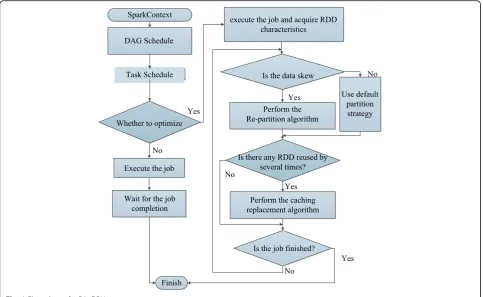
In this section, a parallel acceleration DBN strategy (PA_DBN) is proposed to improve the execution
efficiency of the DBN algorithm in Spark, and the detail process of the PA_DBN strategy is shown in Fig.1.
The detail process of PA_DBN strategy is:
Step 1. Initialize the read data path and the number of data partitions. Spark uses RDD’s text file operator to read the data from HDFS to the memory of the Spark cluster.
Step 2. Create an RBM training method, which contains backpropagation; the result of the backward calculation is used as the next RBM input data, and the weight of DDBN algorithm is updated forward to reduce the error.
Step 3. If data skew occurs, perform the RP algorithm; the re-partition (RP) algorithm is used to partition RDD to avoid the situation that some RDD has much larger size and leads to higher computation time. Step 4. If there is any RDD with reused frequency more
than 2, the RDD cache (RC) algorithm will be performed, which is used to cache frequently reused RDD with higher weight on the basis of the RDD frequency and RDD size. When memory space is insufficient, the RDD with smaller weight will be replaced first.
Step 5.The weight parameter is initialized, the weight of the first layer is calculated, and the weight of the hidden layer is calculated in combination with the function of DBN training in step 2, and then the weight values of each node are merged.
Step 6. Save the weight parameters to HDFS by training.
3.1 Re-partition algorithm
In Spark, the RDD partition is partitioned according to the hash partition algorithm, which results in the different size of the RDD partition in DBN. Based on Definition 3, the maximum partition execution time of RDD deter-mines the execution time of RDD. Therefore, the different size of RDD partition affects the execution speed of DBN. RP algorithm is proposed to solve the problem of data skew caused by skew partitioning of data.
The details of the RP algorithm are:
Step 1.The sample data set is sampled on a small scale, and the sample set is judged to determine whether the data is skewed or not.
Step 2. If the data is skewed, repartition the data. By a series of segmentation tags, if the data hasn partitions based on the parallelism degree, then we need to haven−1 segmentation tags (s1,s2,...,sn−1).
Step 3. When the data is partitioned under Spark, the data is distributed to different partitions according to the tag set, such as key1<s1,s2< key2<s3,...,sn-2
3.2 RDD cache algorithm
In the process of PA_DBN execution, by minimizing the space occupied by the storage area and reserving the memory space allocated to the execution area, the task execution efficiency can be effectively improved. The memory area minimization algorithm is shown in Algo-rithm 1, and the specific steps are as follows:
Step 1. Information of RDDs are obtained from DAG graph of the DBN job. Through pruning analysis and depth-first access, the RDD with action operation is set as the root node, RDDs with the frequency of 0 is pruned, while RDD with frequency more than 1 is re-served as the alternatives. Whenf= 0, delete is no longer used; whenf> 0, the higher the frequency, the
greater the weight of caching. Traversing the key-value pair setR< RDDi,f>, putting the RDD off> 1 into the candidate list to be cached. The dynamic fre-quencyfdecreases by 1 for each RDD visited. Step 2. In actual execution, once the generated RDDs are
in the alternative cache list, they should be compared. If there are more than one RDDs in the candidate list, it is sorted by relative value/size and placed in the cache. The restriction is that the size of RDD and the currently used storage area cannot exceed the allocated storage memory size.
Step 3. When the memory space is insufficient, the least weighted RDDs are cleaned and replaced in turn according to the order of the weight list until the size of the space required by the new RDD is satisfied.
Fig. 2Remote sensing image of Manasi County, Xinjiang
Table 1Different combination of characteristics
Testing set name Parameter
Sample 1 NDVI + RVI + DVI
Sample 2 NDVI + RVI + EVI
Sample 3 NDVI + DVI + EVI
Sample 4 RVI + DVI + EVI
Sample 5 NDVI + RVI + DVI + EVI
4 Result and discussion 4.1 Experimental environment
The experimental environment uses one master and four workers to establish a spark cluster. Considering the large amount of computation and abundant information of re-mote sensing image data, rere-mote sensing image data is used as a data source in this experiment, and the data is derived from a Landsat8 satellite in 2013. The study area is Manas County, Xinjiang, located at 85.7–86.7° E and 43.5–45.6° N (Fig.2). In this paper, the pre-processing of remote sensing data is realized by using ENVI5.2 software to improve the authenticity of remote sensing data. Then
common feature indexes are extracted, such as normalized vegetation index (NDVI), difference vegetation index (DVI), ratio vegetation index (RVI), and enhanced vegeta-tion index (EVI). Based on the four characteristic index parameters, five different text sample sets are extracted as shown in Table1. The other data in the sample set include desert, river, and so on; the training samples and testing samples in grassland; and others are 5000 and 3000 item as shown in Table2.
Table 2Training samples and testing samples
Category Training samples Testing samples
Grassland 5000 3000
Others 5000 3000
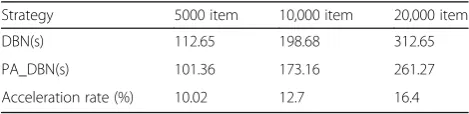
Table 3The execution time of PA_DBN and DBN
Strategy 5000 item 10,000 item 20,000 item
DBN(s) 112.65 198.68 312.65
PA_DBN(s) 101.36 173.16 261.27
4.2 The execution time of PA_DBN
In this experiment, sample 1 is selected as the training set of PA_DBN model. Under the two orders of magni-tude of 5000, 10,000 and 20,000, the test time of PA_DBN and traditional DBN training data is shown in Table3 and Fig.4, where 1, 2, and 3 represent the item of 20,000, 10,000, and 5000 in Fig.3.
Table 3 and Fig. 3 show that the execution speed of
the PA_DBN algorithm is 12.7% times faster than that of the DBN algorithm under the same data volume com-pared with that of the DBN algorithm under the same amount of 10,000 item. In the same amount of 20,000 item, the execution speed of the PA_DBN algorithm is about 16.4% times higher than that of the DBN algo-rithm under the same data volume.
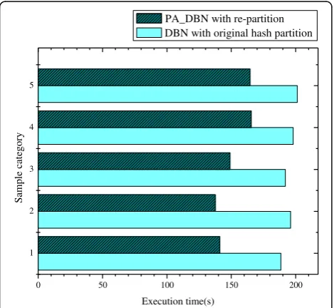
4.3 The execution time by using RP algorithm
With the hidden layer number 3 of DBN, different sam-ples are used for input data, that is, different feature se-lection. The comparison of execution time between the original hash partition and re-partition algorithm is
shown in Fig. 4 by processing the same sample set,
where the number of sample category represents sample 1–5.
In Fig. 4, it can be seen that under different sample sets, the execution speed of PA_DBN is different, and the execution speed of PA_DBN is improved by using the re-partition algorithm. At the same time, the execu-tion time of PA_DBN varies.
Different feature combinations are used as DBN input data, such as NDVI, RVI, DVI, and EVI to test the ac-curacy. When the number of hidden layers of DBN is 3 and the number of iterations is 1000, the other parame-ters are configured fixed. When different feature combi-nations are used as output parameters, the accuracy of
DBN for grassland discrimination is shown in Table 4.
For model structure n-h-o, n represents the number of characteristics,hrepresents the number of hidden layer,
andorepresents the number of output.
In Table4, we could obtain that different feature com-binations are used as input parameters so that the accur-acy of DBN is different; when the feature combination of 1
Fig. 3The comparison with the two algorithms
1 DBN with original hash partition
Fig. 4The comparison by taking a re-partition algorithm
Table 4Different characteristics combination
Characteristic selection Accuracy rate (%) Model structure
NDVI + RVI + DVI 94.92 3-3-2
The number of hidden layer PA_DBN with RC
DBN with LRU
input parameters is NDVI + RVI + DVI + EVI, the high-est accuracy is 96.19.
4.4 The execution time of RC algorithm
In this experiment, the fifth sample set is selected as the training set of the PA_DBN algorithm. By adjusting the number of hidden layers to increase the number of cache RDD, the execution time of RDD before and after using the RC algorithm is tested, as shown in Fig.5.
As shown in Fig.5, by using RC algorithm, the execu-tion time of PA_DBN algorithm for data training is short-ened, and the execution efficiency of PA_DBN algorithm speeds up. Meanwhile, the execution time of both PA_DBN with RC and DBN is increased with the increase in the number of hidden layers, and improving the execu-tion efficiency of DBN becomes more and more signifi-cant. In order to further improve the accuracy of DBN, we test the accuracy of PA_DBN under a different number of hidden layers. The feature combination of NDVI, RVI, DVI, and EVI is used as the input data, iteration times
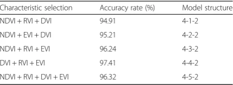
1000. The accuracy of PA_DBN was shown in Table5.
In Table5, it can be seen that the difference in a topo-logical structure is the difference of the corresponding number of hidden layers. As the number of hidden layers increased, the accuracy of PA_DBN for grassland discrimination showed an upward trend. The highest ac-curacy rate of PA_DBN for grassland discrimination was 97.41, and the accuracy of PA_DBN decreased when the number of hidden layers was more than four layers. Therefore, the accuracy of DBN does not increase as the number of hidden layers increases indefinitely.
From Tables2,3, and4and Figs.4and5, there are three groups of experiments in this section. Experiment 1 shows that the training speed of the PA_DBN algorithm is better than that of DBN algorithm under the same order of mag-nitude. Experiment 2 verifies that the RP algorithm is used to solve the problem of data skew and improve the speed of PA_DBN execution. Experiment 3 verifies that the RC al-gorithm is used to solve the problem of high automatic cache re-usability without fine-grained data replacement.
5 Conclusions
In this chapter, we proposed a PA_DBN strategy under Spark to solve some problems existing in the implemen-tation of DBN algorithm on the basis of the theoretical
analysis, such as data skew, lack of fine-grained data re-placement, and high automatic cache re-usability. These problems lead to the defects of high complexity and low execution time of DBN. The parallel acceleration strat-egy based on Spark DBN is adopted to solve the prob-lems. The execution efficiency of PA_DBN strategy is improved, and the training sample is solved by a re-partition algorithm. The problem of skew of this set makes the amount of data contained in each partition of RDD more uniform and improves the speed of DBN training. Through the RC algorithm, it can cache the RDDs with high reused frequency in the DBN algorithm. The experiments are conducted to verify the effective-ness of the presented strategy.
Our future work is mainly concentrated on the follow-ing aspects: analyze different types of remote sensfollow-ing re-sources, design the optimization strategy adapting to the load and type of jobs, and take advantages of another convolutional algorithm to improve the execution efficiency.
Abbreviations
CNN:Convolutional neural network; DAG: Directed acyclic graph; DBN: Deep belief network; RBM: Restricted Boltzmann machines; RDD: Resilient distributed dataset; RS: Remote sensing
Acknowledgements
The authors would like to thank the reviewers for their thorough reviews and helpful suggestions.
Funding
This paper was supported by the National Natural Science Foundation of China under Grant Nos. 61262088, 61462079, and 61562086.
Availability of data and materials
All data are fully available without restriction.
Authors’contributions
CTY is the main writer of this paper. She proposed the main idea, completed the experiment, and analyzed the result. CYY and ZH gave some important suggestions for this paper. All authors read and approved the final manuscript.
Competing interests
The authors declare that they have no competing interests.
Publisher’s Note
Springer Nature remains neutral with regard to jurisdictional claims in published maps and institutional affiliations.
Author details
1School of Mechanical and Electrical Engineering, Shaoxing University, Shaoxing 312000, People’s Republic of China.2School of Information Science and Engineering, Xinjiang University, Urumqi 830008, People’s Republic of China.
Received: 30 July 2018 Accepted: 18 September 2018
References
1. W.S. John, Big data: a revolution that will transform how we live, work, and think. International Journal of Advertising33(1), 181–183 (2014) 2. K. Kambatla, G. Kollias, V. Kumar, et al., Trends in big data analytics. Journal
of Parallel and Distributed Computing74(7), 2561–2573 (2014) Table 5Different number of hidden layer
Characteristic selection Accuracy rate (%) Model structure
NDVI + RVI + DVI 94.91 4-1-2
NDVI + EVI + DVI 95.21 4-2-2
NDVI + RVI + EVI 96.24 4-3-2
DVI + RVI + EVI 97.41 4-4-2
3. C.L.P. Chen, C.Y. Zhang, Data-intensive applications, challenges, techniques and technologies: a survey on big data. Information Sciences275(11), 314–347 (2014)
4. L. Zhang, L. Zhang, B. Du, Deep learning for remote sensing data: a technical tutorial on the state of the art. IEEE Geoscience & Remote Sensing Magazine4(2), 22–40 (2016)
5. M. Das, S.K. Ghosh, Deep-STEP: a deep learning approach for spatiotemporal prediction of remote sensing data. IEEE Geoscience & Remote Sensing Letters13(12), 1984–1988 (2016)
6. G. Hinton, L. Deng, D. Yu, et al., Deep neural networks for acoustic modeling in speech recognition: the shared views of four research groups. IEEE Signal Processing Magazine29(6), 82–97 (2012)
7. V. Badrinarayanan, A. Kendall, R. Cipolla, et al., SegNet: a deep convolutional encoder-decoder architecture for image segmentation. IEEE Transactions on Pattern Analysis and Machine Intelligence39(12), 2481–2495 (2017) 8. L. Mou, P. Ghamisi, X. Zhu, et al., Deep recurrent neural networks for
hyperspectral image classification. IEEE Transactions on Geoscience and Remote Sensing55(7), 3639–3655 (2017)
9. G.E. Dahl, D. Yu, L. Deng, et al., Context-dependent pre-trained deep neural networks for large-vocabulary speech recognition. IEEE Transactions on Audio, Speech, and Language Processing20(1), 30–42 (2012)
10. Y. Chen, X. Zhao, X. Jia, et al., Spectral–spatial classification of hyperspectral data based on deep belief network. IEEE Journal of Selected Topics in Applied Earth Observations and Remote Sensing8(6), 2381–2392 (2015) 11. A. Fischer, C. Igel, Training restricted Boltzmann machines. Pattern
Recognition47(1), 25–39 (2014)