Deep Learning Applications in Medical Image and Shape Analysis

University of Wisconsin Milwaukee

UWM Digital Commons

May 2019

Deep Learning Applications in Medical Image and

Shape Analysis

JINGTAO YANG

University of Wisconsin-Milwaukee

Follow this and additional works at:https://dc.uwm.edu/etd

Part of theComputer Sciences Commons

This Thesis is brought to you for free and open access by UWM Digital Commons. It has been accepted for inclusion in Theses and Dissertations by an authorized administrator of UWM Digital Commons. For more information, please [email protected].

Recommended Citation

YANG, JINGTAO, "Deep Learning Applications in Medical Image and Shape Analysis" (2019).Theses and Dissertations. 2144. https://dc.uwm.edu/etd/2144

DEEP LEARNING APPLICATIONS IN MEDICAL IMAGE

AND SHAPE ANALYSIS

by

Jingtao Yang

A Thesis Submitted in Partial Fulfillment of the Requirements for the Degree of

Master of Science in Computer Science

at

The University of Wisconsin-Milwaukee May 2019

ii

ABSTRACT

DEEP LEARNING APPLICATIONS IN MEDICAL IMAGE AND SHAPE ANALYSIS by

Jingtao Yang

The University of Wisconsin-Milwaukee, 2019 Under the Supervision of Professor Zeyun Yu

Deep learning is one of the most rapidly growing fields in computer and data science in the past few years. It has been widely used for feature extraction and recognition in various applications. The training process as a black-box utilizes deep neural networks, whose parameters are adjusted by minimizing the difference between the predicted feedback and labeled data (so-called training dataset). The trained model is then applied to unknown inputs to predict the results that mimic human's decision-making. This technology has found

tremendous success in many fields involving data analysis such as images, shapes, texts, audio and video signals and so on. In medical applications, images have been regularly used by physicians for diagnosis of diseases, making treatment plans, and tracking progress of patient treatment. One of the most challenging and common problems in image processing is

segmentation of features of interest, so-called feature extraction. To this end, we aim to

develop a deep learning framework in the current thesis to extract regions of interest in wound images. In addition, we investigate deep learning approaches for segmentation of 3D surface shapes as a potential tool for surface analysis in our future work. Experiments are presented and discussed for both 2D image and 3D shape analysis using deep learning networks.

iii

© Copyright by Jingtao Yang, 2019 All Rights Reserved

iv

To My parents,

v

TABLE OF CONTENTS

LIST OF FIGURES ... vii

LIST OF TABLES ... viii

LIST OF ABBREVIATIONS ... ix

Acknowledgements ... x

Chapter 1 ... 1

Introduction ... 1

1.1. Background and Problem Statement ... 1

1.2. Convolutional Neural Network ... 2

1.3. Convolutional Neural Network Architecture ... 3

1.4. Computation of Convolutional Neural Networks ... 7

Chapter 2 ... 10

Wound Analysis with Fully Convolutional Networks ... 10

2.1. Medical Problem Statement ... 10

2.2. Introduction to Fully Convolutional Networks ... 10

2.3. Structure of Fully Convolutional Networks ... 11

2.3.1. Convolution ... 12

2.3.2. Up-sampling ... 13

2.3.3. Skip Architecture ... 14

2.4. Database and Image Label ... 15

2.5. Network Structure ... 18

2.6. Experiments and Analysis ... 19

2.7. Conclusion... 22

Chapter 3 ... 24

CNN Application In 3D Medical Image ... 24

3.1. Problem Statement ... 24

3.2. Description of SPLATNet ... 25

3.2.1. Permutohedral Lattice ... 26

3.2.2. Bilateral Convolution Layer ... 27

3.3. The Structure of SPLATNet ... 28

3.4. Database and 3D Image Label ... 30

vi

3.6. Conclusion... 38

Chapter 4 ... 40

Conclusions and Future Work ... 40

4.1. Conclusions of Medical Image Application ... 40

4.2. Future Work... 41

vii

LIST OF FIGURES

Figure 1 Receptive Field ... 4

Figure 2 Feature Map ... 5

Figure 3 Full Connection Layer Calculation ... 6

Figure 4 Full Connection Layer Transform to Convolution Layer ... 13

Figure 5 Deconvolution ... 14

Figure 6 Labeled Wound Image 1,2 ... 15

Figure 7 Labeled Wound Image 3,4 ... 16

Figure 8 Image Augmentation ... 17

Figure 9 Training Structure ... 18

Figure 10 Residual Block ... 19

Figure 11 Wound Segmentation Result 1 ... 20

Figure 12 Wound Segmentation Result 2 ... 20

Figure 13 Splat Operation ... 26

Figure 14 Bilateral Convolution Layer Process ... 27

Figure 15 Structure of SPLATNet ... 29

Figure 16 Hypercolumn Operation ... 30

Figure 17 Tooth Point Clouds ... 31

Figure 18 Tooth Point Clouds After Processed ... 32

Figure 19 Point Cloud Images of Some Teeth. ... 33

Figure 20 Accuracy of Training ... 34

Figure 21 loss of Training ... 34

Figure 22 Accuracy of Testing ... 35

Figure 23 loss of Testing ... 35

Figure 24 Front View of Testing Sample ... 36

Figure 25 Back View of Testing Sample ... 36

Figure 26 Mesh Graph Transfer to Graph Structure ... .42

Figure 27 Convolution Transform from Graph ... 43

Figure 28 Pooling Operation for Graph ... 44

viii

LIST OF TABLES

ix

LIST OF ABBREVIATIONS

FCN– Fully Convolutional Networks

SPLATNet – SParse LATtice Network

x

ACKNOWLEDGEMENTS

I would like to extend my gratitude to Professor Zeyun Yu as my advisor. Under his professional guidance, I completed the selection of the experimental direction of this paper and conducted in-depth research. His help provided me with a necessary environment and research data for the realization of thesis research, which enabled me to gain some results in this direction, and eventually successfully complete the work in the paper.

I would also like to thank Professor Rohit Kate and Professor Sandeep Gopalakrishnan for joining my thesis committee and give me guidance in their fields of expertise to improve my thesis.

At the same time, I also thank Zhuoran Hao and Chuanbo Wang. The platform they built enabled me to carry out my experiments smoothly and to provide assistance under different experimental requirements.

Finally, I would like to thank my family. Their support and dedication enabled me to complete research and finish thesis writing.

1

Chapter

1

Introduction

1.1.

Background and Problem Statement

As the first step of medical image processing, medical image segmentation plays a key role by extracting regions of interest in medical images and providing more intuitive medical information compared with raw images. In addition, the results of image segmentation can be used for subsequent processing and other research such as quantification and visualization. Traditional segmentation algorithm has one-sidedness in capturing image information and there are some limitations for image segmentation with large differences.

In recent years, with the rise of artificial intelligence research and the warming up of in-depth learning research, Convolutional Neural Network (CNN) [1,2,25,26] has attracted tremendous attention in image processing. Its high efficiency for feature extraction and the special classification model generated by learning make it highly accurate for image

classification. Convolutional neural network has achieved great success in two-dimensional image classification, but it needs a lot of extra effort to be used in two-dimensional and three-dimensional images segmentation.

Three-dimensional images have many forms of data, such as point sources, grids, etc. Different data forms require different processing methods to adapt CNN networks to achieve better segmentation results.

2

1.2.

Convolutional Neural Network

CNN is a multi-layer neural network. Its main feature is that its front-end input uses several layers of locally interconnected neurons to extract image information. A small part of the image is the input of the lowest layer neurons of the hierarchical structure. The information is then transmitted to different layers in turn. Each layer's neurons obtain the most significant features of the observed data through a digital filter.

It fully considers the invariance of translation, rotation and scaling of image objects in space. Its neurons are designed to consist of the same structure, and only accept input from a few neurons in the corresponding field from the previous layer. This design makes the neural network not only maintain a large front-end scale, but also have relatively few variable adjustment parameters, which reduce the computational load and the burden of parameter optimization.

Compared with the manual image pre-processing filtering and convolution process, CNN maintains a relatively low computational complexity while the input image signal size remains unchanged, and its front-end processing process has been optimized. Its weight sharing network structure reduces the complexity of the network model and the number of weights. Feature extraction has the specificity for image content, so its performance is better than that of manual pre-processing, and the recognition effect is much higher than that of traditional methods [3,4].

CNN is one of the most successful deep neural networks. Through the design of hidden layers in the network, the function and form of the layer are changed to better adapt to information processing, and it is widely used in image recognition.

3

1.3.

Convolutional Neural Network Architecture

The hierarchy of convolutional neural networks is divided into five parts:

⚫ Data input layer ⚫ _{Convolutional Layer} ⚫ _{Incentive Layer} ⚫ _{Pooling layer}

⚫ _{Full Connection Layer}

The general CNN consists of a data input layer, multiple convolution layers, excitation layers, pooling layers and full connection layers, and finally outputs the results. Different CNN

structures come from the design, arrangement and number of data input layer, convolution layer, incentive layer, pooling layer and full connection layer to achieve different classification purposes.

The data input layer mainly preprocesses the original image data. In the CNN input layer, the format of the image data input retains the structure of the picture itself. For gray-scale images, the input of CNN is an array of two-dimensional neurons corresponding to image pixels. When considering color images, each color channel of the image has a matrix to form three-dimensional neurons.

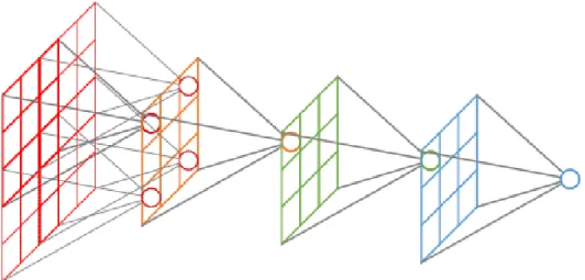
The convolution layer is the most important layer of CNN. There are two important concepts in convolution layer: local receptive fields and shared weights. As shown in Figure 1, the receptive field refers to the area size of the pixels on the feature map output by each layer mapped on the original image. The size of the receptive field is related to the filter size and step size of all previous layers.

4

Each layer has a fixed-size receptive field to capture some of the features of the upper layer. Other features of the upper layer can be obtained by translating the receptive field to other neurons in the same layer. Each neuron is only connected with some of the neuron nodes in the former layer. The weight matrix of thereceptive field is called convolution kernel. Each

receptive field has a convolution kernel, and the scanning interval between the receptive field and the input is called stride. When the stride is larger than 1, the receptive field may be "out of bounds” to scan some features of the edge. At this time, it is necessary to expand the pad,

which can be set as 0 or other values.

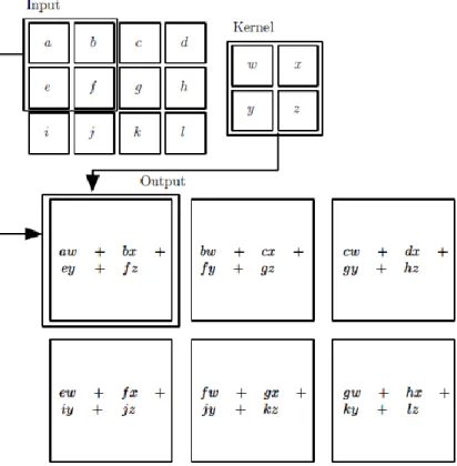
The values of the weight matrix of the convolution kernel are the parameters of the CNN. The convolution kernel may be accompanied by an offset term. In the convolution layer, the weight of each neuron connecting to the data window is fixed, and each neuron pays attention to only one feature. The next neuron matrix generated by a receptive field scan with a

convolution kernel is called a feature map, as shown in Figure 2. The neurons on the same feature map use the same convolution nucleus, so these neurons share the weights and the

5

accompanying offsets in the convolution nucleus. Different feature maps will be obtained if different convolution kernels are used.

The excitation layer maps the output of the convolution layer nonlinearly. The excitation function used is generally ReLu function. The convolution layer and the excitation layer are usually combined and called "convolution layer".

The pool layer lies between continuous convolution layers, often after the convolution to compress parameter. When the input passes through the convolution layer, if the receptive field is small and the stride is small, the result feature map will be large. There are a lot of useless or repetitive information in these feature maps, which affects the accuracy of the next

6

step. At this time, the pooling layer is needed to do the dimension reduction operate on each feature map to remove redundant information and extract the most important features. The information left behind is the most expressive feature of the image, with scale invariance. Currently, the depth of feature map remains unchanged, and the number of feature maps remains unchanged.

Full connection layer is at the tail of convolution neural network, which is used to re-fit features and reduce the loss of feature information. After processing and calculating the data of the full connection layer, the two-dimensional matrix is compressed into one dimension. As shown in Figure 3, the final output classification function is obtained by Softmax function operation.

7

1.4.

Computation of Convolutional Neural Networks

The calculation process of CNN is the same as that of deep learning network. First, the convolution kernels and offset terms are set in the convolution layer and the full connection layer, and then forward propagation is carried out to obtain a calculation result. Then the loss function is used to get the loss between the calculation result and the set result. The

convolution kernel and the offset term are updated by gradient descent method to carry out back propagation. When the convolution kernel and the offset term are less than the iteration threshold, the output network is generated.

In the forward propagation of CNN, the key points are forward propagation of input layer, forward propagation of convolution layer, forward propagation of pooling layer and forward propagation of full connection layer.The forward propagation of input layer and convolution layer is similar, and the process can be expressed as follows:

𝑎2 = 𝜎(𝑧2) = 𝜎(𝑎1∗ 𝑊2+ 𝑏2) (1) Where the superscript represents the number of layers, b represents the bias, the asterisk represents the convolution and σ is the activation function.W Represents Convolutional Kernel Matrix. 𝑎2shows the second layer in CNN, 𝑊2 shows the second layer’s Convolutional Kernel

and 𝑏2 shows the bias parameter of second layer’s Convolutional Kernel.

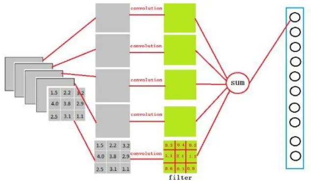
Generally, there are more than one Convolution Kernel in the second layer, such as K, the output of the input layer, or the input of the second convolution layer has K, and the calculation of each Convolution Kernel yields one output.

8

The forward propagation of convolution layer is different from that of input layer. It has M matrices corresponding to the input. Its operation is the sum of the corresponding positions of M matrices after convolution. The process can be expressed as follows:

𝑎𝑙 = 𝜎(𝑧𝑙) = 𝜎(∑𝑀_𝑘=1𝑧_𝑘𝑙) = 𝜎(∑𝑀_𝑘=1𝑎𝑙−1_𝑘 ∗ 𝑊_𝑘𝑙+ 𝑏𝑙) (2) The forward propagation of the pooling layer is to reduce and generalize the input matrix. Generally, the value of the pooling area is reduced to a parameter by MAX or Average method, reduce output as a whole.

The forward propagation of the full connection layer is the same as that of deep learning. For the backpropagation of each layer, the main purpose is to update the convolution kernel matrix parameters and offset term parameters of each layer.

For the fully connected layer, it is deduced as：

𝛿𝑖,𝑙 _{= (𝑊}𝑙+1₎𝑇_𝛿𝑖,𝑙+1_{⊙ 𝜎}′_(𝑧𝑖,𝑙_{) (3)} where 𝛿𝑖,𝑙 represents gradient error calculated by loss function in the ith _{feature map of layer L.}

⊙ represents Hadamard product. So, we can get convolution kernel matrix parameters and offset term parameters as:

𝑊𝑙 = 𝑊𝑙− 𝛼 ∑𝑚_𝑖=1𝛿𝑖,𝑙(𝑎𝑖,𝑙−1)𝑇, 𝑏𝑙 = 𝑏𝑙− 𝛼 ∑𝑚_𝑖=1𝛿𝑖,𝑙 (4) where α represents the iteration step length.

The reverse propagation of convolution layer is like that of full connection layer. it is deduced as：

9

where 𝑟𝑜𝑡180(𝑊𝑙+1) represents the convolution kernel is flipped up and down once, then left and right once, to simplify parameter deduction. So, we can get convolution kernel matrix parameters and offset term parameters as:

𝑊𝑙 = 𝑊𝑙− 𝛼 ∑𝑚_𝑖=1𝛿𝑖,𝑙∗ 𝑎𝑖,𝑙−1, 𝑏𝑙 = 𝑏𝑙− 𝛼 ∑𝑚_𝑖=1 ∑_𝑢,𝑣(𝛿𝑖,𝑙)𝑢,𝑣 (6) The input is pooled by MAX or Average when the pooled layer propagates forward. For the back propagation, the gradient error is reduced from the reduced gradient error 𝛿𝑖,𝑙 to the gradient error corresponding to the pre-pooled region.

Firstly, it is needed to restore the matrix size of 𝛿𝑖,𝑙 to the size before pooling. Then we need to restore it by up-sample process according to the corresponding pooling method. If it is pooling by MAX method, we need to place the corresponding value of 𝛿𝑖,𝑙 according to the position where the maximum value is located. The process can be expressed as follows:

𝛿𝑖,𝑙 = 𝑢𝑝𝑠𝑎𝑚𝑝𝑙𝑒(𝛿𝑖,𝑙+1) ⊙ 𝜎′(𝑧𝑖,𝑙) (7) Where up-sample () represents the reduction method of the corresponding pooling

10

Chapter 2

Wound Analysis with Fully Convolutional Networks

2.1.

Medical Problem Statement

Medical images play an important role in patient diagnosis and treatment. In particular, medical image segmentation is widely applicable in medical research, clinical diagnosis, pathological analysis, surgical planning, image information processing, computer-assisted surgery and other medical research and practice fields. Wound image segmentation is particularly challenging due to complicated types of wounds caused by different reasons. Traditional manual segmentation is laborious, and the segmentation results depend on the operator's experience and knowledge. The manual segmentation results are difficult to reproduce. Traditional algorithms [5-7] are difficult to achieve high accuracy of wound

segmentation. Using the powerful feature extraction ability of deep learning network [8,9], the generalized segmentation of wound images is applied. Because the final outputs of image results are needed for image segmentation, FCN [8] is used to study the wound segmentation problem in the current thesis.

2.2.

Introduction to Fully Convolutional Networks

CNN has been driving the progress of image recognition. Whether it is the classification of the whole picture [2,25,26] or the object detection [27-29], the key point detection has been greatly developed with the help of CNN. But image semantics segmentation is different from

11

the above tasks. It is a space-intensive prediction task. In other words, it needs to predict the categories of all the pixels in an image.

Generally, CNN networks connect several full-connection layers after the convolution layer, mapping the feature map generated by the convolution layer into a fixed-length feature vector, obtaining a numerical probability of the whole input image, and classifying it.

Unlike classical CNN, which uses full-connection layer to get fixed-length feature vectors after convolution layer for classification (full-connection layer + soft Max output), Fully

Convolutional Networks (FCN) can accept any size of input image and uses deconvolution layer to sample feature map of the last convolution layer to restore it to the same size of input image, so that each pixel can be generated. At the same time, the spatial information of the original input image is retained. Finally, the pixel-by-pixel classification is carried out on the feature map sampled above.

2.3.

Structure of Fully Convolutional Networks

Compared with CNN, most of the structures of FCN are the same. The difference is that CNN needs to compress the matrix into one dimension in the full connection layer and complete the classification by classifier. FCN replaces the full connection layer with convolution layer to restore the image and get the image segmentation result. There are three parts involved: convolution, up-sampling and Skip Architecture.

12

2.3.1.

Convolution

The only difference between the full connection layer and the convolution layer is that the neurons in the convolution layer connect only to a local area of the input data and share parameters with the neurons in the convolution column. However, in both layers, neurons compute point product, so their function forms are the same.

So, the full connection layer can be transformed into convolution layer. For example, in a fully connected layer with a value of K, the size of input data is M *M *L, and the fully

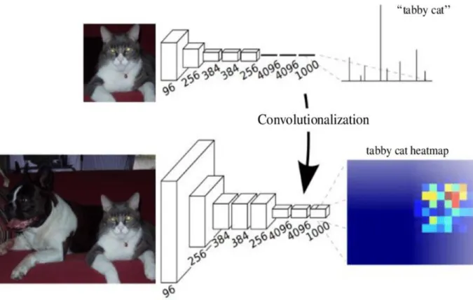
connected layer can be regarded as a convolution layer with K convolution kernels of M*M size, filling value of 0 and strike size of 1. Set the size of the filter to be the same as the size of the input data. Because only one depth column covers and skips over the input data, the output will become 1*1*K, which is the same as using the original full connection layer, as shown in Figure 4.FCN converts the last three full connection layers into three convolution layers with the size of 1*1*4096, 1*1*4096, 1*1*1000.

After many convolutions and pooling, the image is getting smaller and smaller, and the resolution is getting lower and lower. When the image reaches the smallest level, the

generated image is called Heatmap, which is the most important high-dimensional feature map. Then up-sampling the Heatmap and enlarging the image to the size of the original image.

13

2.3.2.

Up-sampling

In general CNN structure, pooling layer is used to reduce the size of the output image. What we need is a segmented image with the same size as the original image, so we need to sample the last layer up.

Up-sampling has a variety of methods, such as interpolation method, anti-pooling method, etc. In FCN, deconvolution method is generally used to amplify. The forward propagation process of deconvolution is like the reverse propagation process of convolution layer, as shown in Figure 5. Firstly, the input matrix is expanded, and then the results larger than the input

Figure 4 Full Connection Layer Transform to Convolution Layer https://www.researchgate.net/figure/Converting-fully-connected-layers-of-CNN-to-convolutional-layers-20_fig14_327260166

14

matrix are calculated according to the convolution layer calculation method, and the up-sampling operation is completed.

2.3.3.

Skip Architecture

Usually the first two methods are used directly to get the original image, but the result of the original image is very rough. So, skip structure is needed to optimize the result.The idea is to sample the results of different pooling layers in the original CNN, and then optimize them with different weights to get better results.

Through the above methods, combined with CNN structure, the segmentation results of original image size can be obtained.

15

2.4.

Database and Image Label

The wound image chosen from the Medetec Wound Database. It contains pictures of many types of open wounds that are often encountered by wound care practitioners. The types of wound in this dataset include venous leg ulcers, arterial leg ulcers, pressure ulcers, malignant wounds, dehiscent wounds caused by surgical wound infections, skin or microvascular changes associated with diabetes, diabetic ulcers, ischemic wounds and other wound types.

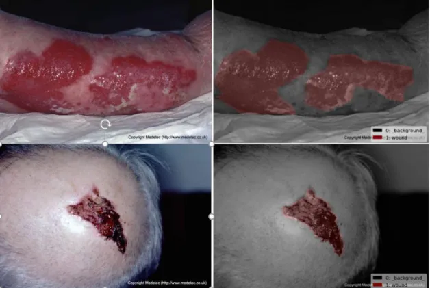
Among them, 390 pictures were selected to construct the training dataset. By using the label-me program [10], the labeled images are shown in Figure 6, 7.

16

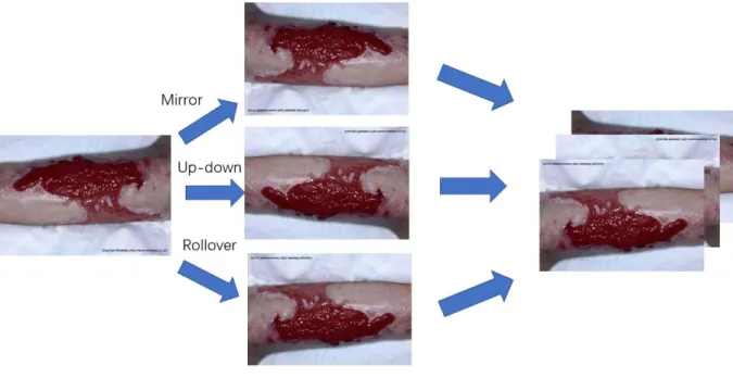
These images are far from enough for deep neural networks. Large-scale datasets are the prerequisite for successful application of deep neural networks. So, it is needed to use image augmentation technology to expand the dataset, as shown in Figure 8. This method generates similar but different training samples by making a series of random changes to the training image, thus enlarging the scale of training data set. These randomly changing training samples can reduce the dependence of the model on some attributes and improve the generalization ability of the model.

17

In this paper, we use up-down flip and left-right flip to achieve image enlargement, and randomly adjust the brightness in these pictures to achieve greater difference and reduce the sensitivity of the picture to color, as shown in Figure 8. Finally, the input pictures are randomly cut to meet the size required for FCN input.

After this process, the total dataset has 1560 images. It contains 1200 images used for training set 360 images used for predicting set.

18

2.5.

Network Structure

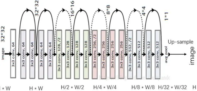
The structure of FCN network used for wound segmentation in this paper is shown in Figure 9. The first half is ResNet-18 [11]. The structure consists of four residual blocks. The first three residual blocks reduce the image length by half. The last residual block reduces the image length to H/32*W/32. After that, the number of channels is transformed into the number of categories through 1*1 convolution layer. Finally, the height and width of the feature map are transformed into the size of the input image by transposing the convolution layer.

In the ResNet-18 [11] structure, the residual block effectively solves the Degradation

problem. When the network depth increases, the network accuracy saturates or decreases due to the disappearance or explosion of the gradient. Residual blocks are shown in Figure 10.

19

2.6.

Experiments and Analysis

This experiment uses MXNET platform to test. The test environment is NVIDIA Corporation GP102 [TITAN Xp]. The evaluation index of image segmentation includes many evaluation criteria. In this experiment, accuracy is chosen as the evaluation criterion, and its formula is as follows:

𝑃𝑟𝑒𝑐𝑖𝑠𝑖𝑜𝑛 = 𝑁𝑇𝑃

𝑁𝑇𝑃+𝑁𝐹𝑃 (8)

The 𝑁_𝑇𝑃 represents the correct number of pixels in the image. The 𝑁_𝐹𝑃 represents the number of pixels marked incorrectly in the image.

The training accurate is about 97%, the test accurate is about 94%. The wound segmentation result is shown as Figure 11, 12.

Figure 10 Residual Block https://towardsdatascience.com/residual-blocks-building-blocks-of-resnet-fd90ca15d6ec

20

Figure 11 Wound Segmentation Result 1

21

In Figures 11 and 12, the left side is the original image, the right side is the marked image, and the middle is the predicted image. Fig. 11 is the prediction result of the same image after data augmentation. Figure 12 shows the test results of different images after training.

As can be seen from Figure 11, rotation augmentation for the same image effectively

increases the difference. It is helpful to enlarge the data and improve the accuracy of the neural network. It can be seen from the comparison of the first four images that when the part of the marked image is less than a certain value, the accuracy of the marking will be greatly reduced, so that the marking cannot be achieved at all. When there is interference background similar to the label content in the image, the neural network cannot eliminate the interference effectively, and there are some errors.

As can be seen from Figure 12, for different types of open wound images, FCN can effectively segment the wound area and ensure the correct rate of large area of wound.

However, there are some errors between the neural network trained by FCN and the marker in the recognition of wound edge. For the second and third image, there are obvious errors in the prediction of the neural network in the image with complex edge conditions, and most of the edge wound markings are neglected. For the fourth and fifth image, the neural network perfectly predicts the wound part and achieves significant wound segmentation judgment. However, there are still slight errors and uncertainties in the edge of the wound.

Overall, FCN achieves the expected wound segmentation, and more data processing and training are needed to achieve higher accuracy on edge issues.

22 2.7.

Conclusion

In the application of FCN in wound image segmentation, the neural network has shown its excellent segmentation ability, which can meet the requirements of effective segmentation of most wound areas in the wound image. But there are still some problems. For example, it is impossible to predict a wound less than a certain range, there are omissions in the detection of edge problems, even for the complex situation of the wound edge, it is impossible to complete the marking, and there are problems in judging the edge of a special wound.

Some of these problems are due to the lack of data resources, which affects the judgment of the neural network in the learning process. Others are due to the poor prediction of the characteristics of the neural network. For FCN, because of the simplified steps in feature

extraction, the neural network ignores some small features which are not obvious. It makes the judgement of these characteristics lost in the training process. The result is not very precise. On the other hand, FCN is a point-to-point prediction, and the result is accurate to every pixel. In the classification of each pixel, the relationship between the pixel and the pixel is not fully considered. The steps of spatial regularization are neglected, which leads to the lack of spatial consistency in image classification.

For the problems of neural network, we can try to solve them by other methods. When too small wounds cannot be segmented, training and prediction can be carried out by enlarging the marked area of the image and reducing the unmarked area. The results can be reduced in equal proportion to achieve the prediction of the original image wound segmentation. In the actual test, some simple segmentation algorithms can be used to estimate the labeling rate, and the

23

image smaller than a certain value can be segmented and enlarged. Restore the image after completing the prediction.

For the problems of edge detection, we can try to reduce background interference and narrow the segmentation area to improve the accuracy of neural network training. In the case of complex edges, the traditional segmentation algorithm can be used to supplement the prediction results. By this way, the accuracy of the results will be improved, and the complexity of the neural network will be reduced.

24

Chapter

3

CNN Applications In 3D Shape Analysis

3.1.

Problem Statement

With the development of scanning technology, it is more and more convenient to construct accurate 3D geometric models of objects. Compared with two-dimensional data,

three-dimensional data has better properties. It has prominent application value in various fields because of its stereoscopic display of images, visualized description of the volume of objects and more details of objects. It visualizes the abstract and difficult spatial information, which is convenient to quickly understand and make accurate judgments.

Three-dimensional shapes have different expressions, such as triangular meshes, point clouds, voxels, parametric surfaces, implicit surfaces, etc. Different expressions have different combinations in the use of CNN. For example, the methods in [12-14, 30-32] project the three-dimensional image into two-three-dimensional space and perform convolution network operations on two-dimensional images from multiple perspectives. Those in [15,16] transform the three-dimensional image into multiple surfaces for convolution network operations. The authors in [17,18,33-36] transform the three-dimensional image into voxels for convolution network operations. In recent years, in the research of vision, machine learning and computer graphics, various deep learning networks for three-dimensional shape have been developed. But these methods have different requirements for data form and time spend.

25

With the development of medical imaging technology and three-dimensional visualization technology, computer-aided diagnosis has become a reality. With the development of

computer technology, doctors and researchers can better understand the structure of human body and diagnose patients through virtual interaction. Three-dimensional shape segmentation plays an important role in the segmentation of regions of interest. In this chapter, the

application of depth neural network is mainly aimed at three-dimensional shape segmentation of teeth. Its ultimate goal is to achieve the segmentation of single different types of teeth, but for the preliminary research stage, the first step is to complete the segmentation of teeth and gingiva.

For this tooth segmentation experiment, we use the original data of three-dimensional point cloud as input. In the training process, we choose a relatively fast training model. Based on the above considerations, SParse LATtice Network (SPLATNet) is chosen as the neural network in this experiment.

3.2.

Description of SPLATNet

SPLATNet [19] is a neural network structure proposed by Hang Su of UMass Amherst to segment point clouds. Its emphasis is on the network constructed with Bilateral Convolution Layer (BCL) [21,22,41,42]. The BCL transforms the input point clouds and convolutes them to get the features. Its purpose is to solve the spatial relationship in point clouds and ensure the invariance of point clouds.

26

The BCL maps the input point cloud to the permutohedral lattice and adds the mapped points to the vertices of the simplex using barycentric interpolation method to form a sparse lattice.

3.2.1.

Permutohedral Lattice

Permutohedral lattice [20] is a new coordinate system which is derived from the higher processing speed of Gauss convolution in image processing. When a point is mapped to a permutohedral lattice, the coordinates of the point are not projected to a point in the new coordinate, but to each vertex of a lattice in the new coordinate through the barycentric interpolation. Reserve the weight of each vertex generated by barycentric interpolation to prepare for the restoration of points. If two different points are projected to the same vertex coordinates, increase the value of this point. The operation of mapping points is called splat, and the process is shown in Figure 13.

Figure 13 Splat Operation https://www.slideserve.com/rico/mean-field-theory-and-its-applications-in-computer-vision3

27

3.2.2.

Bilateral Convolution Layer

BCL [21,22,41,42] originates from the generalization of bilateral filtering, which involves projecting a given image into a higher dimensional space with more definitions. Unlike bilateral filtering, which uses custom filtering kernels in high-dimensional space, BCL filtering kernels need to be trained and learned in neural networks. The flow of BCL is shown in Figure 14.

The first step is called Splat. Through barycentric interpolation, point clouds containing input characteristic F are projected to a new coordinate system with lattice characteristic L on permutohedral lattice. The lattice feature ΔL controls the size of the cell or the space between the grid points by scaling, where Δis the scaling matrix of dl*dl.

The second operation is called Convolve. After the Platform operation, the features of the projected points have been allocated to the vertices of each simplex according to certain principles. Therefore, the position of each point in permutohedral lattice is relatively regular.

28

The index is made according to the hash table, and the convolution operation is carried out through the learnable filter kernel.

The last step is called Slice. This part is the reverse operation of Splat, which gathers the information on Lattice vertex from convolution operation in the second part to the original point. The reduction is performed by interpolation coefficients of barycentric interpolation. After convolution operation, the result will be different from the input. These points may appear in new locations, and the number of points may be less than the original points, depending on the filter core. This is like the image size transformation after CNN convolution operation.

The operation of BCL is similar to that of convolution layer in CNN. The difference is that it performs a coordinate change to make convolution easier for sparse points.

3.3.

The Structure of SPLATNet

The SPLATNet used in this experiment is shown in Figure 15. The input point cloud data are processed by the first transformation layer and sampled by five different BCL. For SPLATNet, the XYZ coordinates of points are used as input for BCL. In permutohedral lattice, different lattice spacing is applied to different BCL, resulting in different resolution in convolution operations. The lattice begins with the first BCL, and the lattice spacing of the next BCL is half that of the previous one. After many changes in lattice spacing, the final BCL has the largest effective acceptance field, and there is a long connectivity between the input points. The change of lattice spacing is helpful to extract the features of different spatial sizes and levels.

29

After obtaining the feature maps of BCL at each level, SPLATNet uses the Hypercolumn [23] to get the results obtained at each level. Fine target localization is performed by using the activation series of the obtained feature graph networks as features. The principle is shown in Figure 16.

After extracting features from BCL, each position of the feature map is classified by 1*1 convolution, and the features are divided into blocks corresponding to each feature map, and then the score map is generated by 1*1 convolution for each block. Because of the different sizes of feature maps, bilinear interpolation is needed to scale the feature maps to a uniform size (up-sampling). Finally, all feature maps are accumulated.

After aggregating information in different BCL by series operation, SPLATNet uses two 1*1 convolution layers to transfer data to SoftMax layer and generate classification probability of points. The segmentation of point clouds is predicted by classification probability.

30

3.4.

Database and 3D Image Label

In this experiment, we used the 3D point cloud image of teeth as input. A total of 19 labeled tooth point clouds is obtained. As shown in Figure 17, there are 35 921 dots in this image, of which the blue dot is the tooth part (labeled 1) and the yellow dot is the gingival part (labeled 0).

31

In the tooth point cloud data, there are many points unrelated to the tooth image. In Figure 17, the lower edge structure points are generated by scanning. These points will affect the segmentation of dental images and produce unnecessary errors. Therefore, the point cloud data of the original teeth need to be processed to obtain the point cloud data as shown in Figure 18.The remaining point cloud has 26191 points

Figure 17 Tooth Point Clouds. The top is the point cloud's back view, and the bottom is the point cloud's forward view.

32

Due to insufficient data, we divide a complete set of point cloud images into 3-4 point cloud images containing at least three teeth, as shown in Figure 19. Finally, 57 point cloud images containing only part of the teeth were obtained. Among them, 44 point cloud images are used for training set and 13 point cloud images are used for testing set.

Figure 18 Tooth Point Clouds After Processed. The top is the point cloud's back view, and the bottom is the point cloud's forward view.

33

3.5.

Experiments and Analysis

This experiment uses Caffe platform to test. The test environment is Nvidia Corporation GP102 [Titan XP]. IoU (intersection-over-union) parameters are used in the evaluation of three-dimensional image segmentation. That is to say, the intersection ratio of the detection results and the ground truth is their union. The formula is as follows:

𝐼𝑜𝑈 = 𝐷𝑒𝑡𝑒𝑐𝑡𝑖𝑜𝑛𝑅𝑒𝑠𝑢𝑙𝑡 ∩ 𝐺𝑟𝑜𝑢𝑛𝑑𝑇𝑟𝑢𝑡ℎ

𝐷𝑒𝑡𝑒𝑐𝑡𝑖𝑜𝑛𝑅𝑒𝑠𝑢𝑙𝑡 ∪ 𝐺𝑟𝑜𝑢𝑛𝑑𝑇𝑟𝑢𝑡ℎ (9) The experimental data are trained for 2000 iterations, and the test results are shown in Fig. 20-23.A sample of the predicted results is shown in Figure 24-25, for example. The result is in Table 1.

34

Figure 20 Accuracy of Training lateral axis is iteration, vertical axis is the accuracy, maximum is 1

35

Figure 22 Accuracy of Testinglateral axis is iteration, vertical axis is the accuracy, maximum is 1

36

Figure 24 Front View of Testing Sample. Left is labeled image, right is prediction image

37 Table 1 Experiment Result

Training Accuracy Training Loss Testing Accuracy Testing Loss

81.1% 0.384 77.5% 1.15

Sample Predict Accuracy 62.5%

As can be seen from Figure 20, the accuracy of the training set is gradually increasing, hovering between 76% and 83%. The highest was 83.4%. Then there was a decline in accuracy. From the accuracy of training set, it can be concluded that this neural network is not sufficient for feature extraction of data set. As a result, the expected accuracy is not high, and the

adjustment is not large in the later period. More iterations are needed to improve the accuracy slowly.

As can be seen from Figure 22, the accuracy of the test set fluctuates greatly, reaching 80% at the maximum, and maintaining 76% to 78% at the end. From the accuracy of the test set, it can be concluded that the network parameters trained by the neural network are not enough to judge the test set. In the case of multiple iterations, the accuracy is not very high.

As can be seen from Figure 24-25, the accuracy of segmentation of some 3D point clouds of teeth is not very high. But it can basically separate the teeth and gingiva. There is serious ambiguity in the edge areas of the two parts. As can be seen from Figure 24, in the front point cloud segmentation, the right teeth have a good segmentation effect, and the boundary between the teeth and the teeth has a clear segmentation. There is a significant error between the left tooth and the middle tooth. As can be seen from Figure 25, in the back-point cloud

38

segmentation, there are errors in the gingival segment between teeth and teeth, and there are obvious errors in the lower part of the middle teeth.

3.6.

Conclusion

In this experiment, we used SPLATNet neural network structure to segment teeth and gingiva in the data, using the point cloud data of teeth as input. In the case of existing data, we get a SPLATNet neural network model and test it. From the results, the model trained by the neural network plays a certain role in tooth data segmentation, but the accuracy is not high, and the test results are partitioned, but there are a lot of errors in the edge situation. There are many reasons.

Firstly, the lack of tooth data may result in the inability of better image segmentation due to the problem of data volume. The second possibility is that the point cloud data are missing when the tooth image is re-segmented, which makes the extraction of tooth characteristics inadequate. Thirdly, because of the computer performance, the number of single point cloud data input is too small to better express the characteristics of teeth, which makes the

segmentation misjudged. Fourthly, it may be that the characteristics of point clouds cannot express the shape of teeth better, which leads to the lack of characteristics of point clouds.

For the first guess, more data is needed to support the segmentation of tooth point clouds to improve performance. For the second guess, we can try to train the whole tooth point cloud image and draw a conclusion through comparison. For the third guess, we can try to optimize the performance of the neural network to input more points at the same time. For the fourth guess, we can try to deal with the network data.

39

For the first two problems, more dental data are needed, which can be achieved in subsequent experiments. For the third problem, the difference between the input of point cloud data and the real tooth point cloud data is too large to be realized without improving the performance of the machine. For subsequent tooth segmentation, the single tooth

segmentation becomes an obstacle. So next, we will try to use the neural network to train the grid data and require that there is no size limit for data input. It can input as many data features as possible while ensuring the relevance of data and carry out more refined medical image segmentation.

40

Chapter 4

Conclusions and Future Work

4.1.

Conclusions of Medical Image Application

For medical image segmentation, we try different deep learning neural networks based on convolution neural network. For two-dimensional image segmentation, we choose open wound images as the research object, FCN structure as the application structure, and design the

application of deep learning network through the modification of Resnet-18. In this experiment, Resnet-18 is used to alleviate the performance degradation caused by depth, and the

deconvolution layer in FCN concept is used to realize point-to-point image segmentation. In the problem of three-dimensional image, we choose the available three-dimensional point cloud data to study and segment the three-dimensional point cloud model of teeth in medical images. In the selection of deep learning neural network, we choose SPLANet neural network based on CNN concept. Compared with the traditional CNN model, SPLATNet replaces the original convolution layer with BCL and realizes the transformation and fast convolution of three-dimensional point clouds in Permutohedral Lattice. In the final classification, SPLATNet uses Hypercolumn structure to refine the classification of the output image.

In the experiment, the application of two-dimensional wound image segmentation has played a good role, for most of the wound images can be effectively segmented. For the

41

reached the expectation for various reasons. For the point cloud image of teeth, it can only be roughly segmented, and there are great errors in the boundary part.

4.2.

Future Work

With the development of medical image instruments and imaging, more and more dimensional images have come into our field of vision. After the segmentation of the three-dimensional image, the result can be easily substituted for the segmentation of the two-dimensional image. Therefore, in the future research, we will be more inclined to the application of three-dimensional image segmentation in deep learning network.

For the application of tooth image segmentation in three-dimensional image, the SPLATTNET neural network has not achieved the desired results. In the information of three-dimensional image of teeth, grid information can help us better define the characteristics of teeth. So, in the following research, we will try the deep learning network related to three-dimensional mesh image segmentation [37-40] to continue the research on three-three-dimensional model segmentation of teeth.

In the process of researching the three-dimensional mesh image, [24] shows a good idea that all kinds of meshes in the three-dimensional mesh image can be transformed into

triangular meshes. In a triangle, there are three adjacent triangles besides the edge area. If the triangle is set as a node, the three-dimensional image with the triangle as a grid can be

42

In the graph structure, each node is a triangle. The transformed three-dimensional mesh image can be represented by a two-dimensional graphic structure. It can not only retain the connection relationship between triangles, but also fix the number of connections of each node, which is convenient for calculation. However, in the new graph structure, the triangles

represented by each node lose the shape characteristics of spatial connection, so more

dimensions need to be added to the nodes represented by each triangle to preserve the spatial properties of triangles.

For each node, we can add some advanced attributes to assist the network in judging triangle classification in the model. Such as curvature (CUR) [43], shape diameter function (SDF) [44], shape context (SC) [45], PCA feature (PCA) [46], average geodesic distance (AGD) [47], spin image (SI) [48] and so on.

In the research of CNN for graphical structure, the idea of transforming multiple nodes is put forward. The most important part is how to complete the operation of convolution and the

43

processing of pooling. In [49,50], the application of convolution is mainly transformed by graphical structure, which cannot well represent the characteristics of node triangle. So, we finally choose the node as the pixel point to convolute the node. To ensure the edge connection of triangles, we use each triangle and its three adjacent triangles as a group to convolute and calculate all triangles. Its form is shown in Figure 27.

For the pooling operation, we use the pooling method mentioned in [38,50] to roughen the original graphic structure to maintain the connection relationship after the convolution of the graphic structure. Multilevel clustering algorithm [51] is used to calculate the weights of the corresponding nodes to ensure the relationship between the coarsened nodes and the original graph. To ensure the requirement of graph coarsening, we add some virtual points to keep the total number of triangles in the model consistent. Its form is shown in Figure 28.

44

Through the application of these two parts, the deconvolution reduction operation in FCN and the optimization of Hypercolumn structure are added. CNN for graphical structure can be obtained.

This provides a new classification idea for three-dimensional mesh images, but there are still many unsolved problems. These problems will be solved step by step in the future research, and new neural network attempts will be implemented.

45

References

[1] Yann LeCun, Leon Bottou, Yoshua Bengio, and Patrick Haffner. “ Gradient-based learning applied to

document recognition” . Proceedings of the IEEE, 86(11):2278–2324, 1998.

[2] A. Krizhevsky, I. Sutskever, and G. Hinton. “ ImageNet classification with deep convolutional neural

networks”. In NIPS, 2012.

[3] E. Saber, A.M. Tekalp,”Integration of color, edge and texture features for automatic region-based

image annotation and retrieval,” Electronic Imaging, 7, pp. 684–700, 1998.

[4] O.D. Trier, A.K. Jain and T. Taxt,” Feature extraction methods for character recognition - a survey,”

Pattern Recognition, 29(4), pp. 641–662, 1996

[5]F. Veredas, H. Mesa, and L. Morente, “Binary tissue classification on wound images with neural

networks and bayesian classifiers,” IEEE Transactions on Medical Imaging, vol. 29, no. 2, pp. 410–

427, 2010.

[6] M. K. Yadav, D. D. Manohar, G. Mukherjee, and C. Chakraborty, “Segmentation of chronic wound areas by clustering techniques using selected color space,” Journal of Medical Imaging and Health Informatics, vol. 3, no. 1, pp. 22–29, 2013.

[7] A. K. Bhandari, A. Kumar, S. Chaudhary, and G. K. Singh, “A novel color image multilevel thresholding

-based segmentation using nature inspired optimization algorithms,” Expert Systems with

Applications, vol. 63, pp. 112–133, 2016.

[8] J. Long, E. Shelhamer, and T. Darrell, “Fully convolutional networks for semantic segmentation,” in

Proceedings of the IEEE Conference on Computer Vision and Pattern Recognition (CVPR '15), pp.

3431–3440, IEEE, Boston, Mass, USA, June 2015.

[9] C. Wang, X. Yan, X. Smith et al., “A unified framework for automatic wound segmentation and analysis with deep convolutional neural networks,” in Proceedings of the 2015 37th Annual

International Conference of the IEEE Engineering in Medicine and Biology Society (EMBC '15), pp.

2415–2418, Milan, Italy, August 2015.

[10] B.C. Russell, A. Torralba, K.P. Murphy, and W.T. Freeman. “Labelme: a database and web-based tool

for image annotation”. International journal of computer vision, 77(1):157–173, 2008.

[11] K. He, X. Zhang, S. Ren, and J. Sun, “Deep residual learning for image recognition” in Proceedings of

the IEEE Conference on Computer Vision and Pattern Recognition (CVPR '16), pp. 770–778, Las

Vegas, Nev, USA, June 2016.

[12] H. Su, S. Maji, E. Kalogerakis, and E. G. Learned-Miller. “Multi-view convolutional neural networks

for 3D shape recognition”. In Proc. ICCV, 2015.

[13] C. R. Qi, H. Su, M. Niener, A. Dai, M. Yan, and L. J. Guibas. “Volumetric and multi-view CNNs for

object classification on 3D data”. In Proc. CVPR, 2016.

[14] E. Kalogerakis, M. Averkiou, S. Maji, and S. Chaudhuri. “3D shape segmentation with projective

46

[15] H. Pan, S. Liu, Y. Liu, and X. Tong. “Convolutional neural networks on 3d surfaces using parallel

frames”. arXiv preprint arXiv:1808.04952, 2018

[16] S. B. Seong, C. Pae, and H. J. Park, “Geometric convolutional neural network for analyzing surface

-based neuroimaging data,” Frontiers in Neuroinformatics, vol. 12, p. 42, 2018.

[17] P.-S. Wang, Y. Liu, Y.-X. Guo, C.-Y. Sun, and X. Tong.” OCNN: Octree-based convolutional neural

networks for 3D shape analysis”. ACM Trans. Graph., 36(4), 2017.

[18] Z. Wu, S. Song, A. Khosla, F. Yu, L. Zhang, X. Tang, and J. Xiao. “3D shapenets: A deep representation

for volumetric shapes”. In Proc. CVPR, 2015.

[19] H. Su, V. Jampani, D. Sun, S. Maji, E. Kalogerakis, M.-H. Yang, J. Kautz, "Splatnet: Sparse lattice networks for point cloud processing", Proceedings of the IEEE Conference on Computer Vision and Pattern Recognition, pp. 2530-2539, 2018.

[20] A. Adams, J. Baek, and M. A. Davis. “Fast high-dimensional filtering using the permutohedral lattice”.

Computer Graphics Forum, 29(2):753–762, 2010.

[21] V. Jampani, M. Kiefel, and P. V. Gehler. “Learning sparse high dimensional filters: Image filtering,

dense CRFs and bilateral neural networks”. In Proc. CVPR, 2016

[22] M. Kiefel, V. Jampani, and P. V. Gehler. “Permutohedral lattice CNNs”. In ICLR workshops,May 2015.

[23] B. Hariharan, P. Arbelaez, R. Girshick, and J. Malik. “Hypercolumns for object segmentation and

fine-grained localization”. In Computer Vision and Pattern Recognition, 2015

[24] P. Wang, Y. Gan, P. Shui, F. Yu, Y. Zhang, S. Chen, and Z. Sun. “3d shape segmentation via shape fully

convolutional networks”. Computers & Graphics, 2017

[25] K. Simonyan and A. Zisserman.” Very deep convolutional networks for large-scale image

recognition”. CoRR, abs/1409.1556, 2014.

[26] C. Szegedy, W. Liu, Y. Jia, P. Sermanet, S. Reed, D. Anguelov, D. Erhan, V. Vanhoucke, and A.

Rabinovich. “Going deeper with convolutions”. CoRR, abs/1409.4842, 2014.

[27] P. Sermanet, D. Eigen, X. Zhang, M. Mathieu, R. Fergus, and Y. LeCun. “Overfeat: Integrated

recognition, localization and detection using convolutional networks”. In ICLR, 2014.

[28] R. Girshick, J. Donahue, T. Darrell, and J. Malik. “Rich feature hierarchies for accurate object

detection and semantic segmentation”. In Computer Vision and Pattern Recognition, 2014.

[29] K. He, X. Zhang, S. Ren, and J. Sun. “Spatial pyramid pooling in deep convolutional networks for

visual recognition”. In ECCV, 2014.

[30] S. Bai, X. Bai, Z. Zhou, Z. Zhang, and L. J. Latecki. “GIFT: a real-time and scalable 3D shape search

engine”. In Proc. CVPR, 2016.

[31] Z. Cao, Q. Huang, and K. Ramani. “3D object classification via spherical projections”. In Proc. 3DV,

47

[32] H. Huang, E. Kalegorakis, S. Chaudhuri, D. Ceylan, V. Kim, and E. Yumer. “Learning local shape

descriptors with viewbased convolutional neural networks”. ACM Trans. Graph., 2018.

[33] A. Brock, T. Lim, J. M. Ritchie, and N. Weston. “Generative and discriminative voxel modeling with

convolutional neural networks”. arXiv:1608.04236, 2016.

[34] N. Sedaghat, M. Zolfaghari, E. Amiri, and T. Brox. “Orientation-boosted voxel nets for 3D object

recognition”. In Proc. BMVC, 2017.

[35] G. Riegler, A. O. Ulusoys, and A. Geiger. “Octnet: Learning deep 3D representations at high

resolutions”. In Proc. CVPR, 2017.

[36] R. Klokov and V. Lempitsky. “Escape from cells: Deep KdNetworks for the recognition of 3D point

cloud models”. In Proc. ICCV, 2017.

[37] J. Bruna, W. Zaremba, A. Szlam, and Y. LeCun. “Spectral networks and locally connected networks on

graphs”. In Proc. ICLR, 2014

[38] M. Defferrard, X. Bresson, and P. Vandergheynst. “Convolutional neural networks on graphs with

fast localized spectral filtering”. arXiv:1606.09375, 2016

[39] D. Boscaini, J. Masci, S. Melzi, M. M. Bronstein, U. Castellani, and P. Vandergheynst. “Learning

class-specific descriptors for deformable shapes using localized spectral convolutional networks”. In

Proc. SGP, 2015.

[40] M. Henaff, J. Bruna, and Y. LeCun. “Deep convolutional networks on graph-structured data”.

arXiv:1506.05163, 2015.

[41] V. Aurich and J. Weule. “Non-linear Gaussian filters performing edge preserving diffusion”. In DAGM,

pages 538–545. Springer, 1995.

[42] C. Tomasi and R. Manduchi. “Bilateral filtering for gray and color images”. In Proc. ICCV, 1998.

[43] K. Kavukcuoglu, M. Ranzato, R. Fergus, Y. LeCun. “Learning invariant features through topographic

filter maps”. In: IEEE Conference on Computer Vision & Pattern Recognition. 2009.

[44] R. Liu, H. Zhang, A. Shamir, D. Cohen-Or. “A part-aware surface metric for shape analysis”.

Computer Graphics Forum 2009.

[45] S. SBelongie, J. Malik, J. Puzicha. “Shape matching and object recognition using shape contexts”.

IEEE Transactions on Pattern Analysis & Machine Intelligence 2002.

[46] L. Shapira, S. Shalom, A. Shamir, D. Cohen-Or, H. Zhang. “Contextual part analogies in 3d objects”.

International Journal of Computer Vision 2010.

[47] M. Hilaga, Y. Shinagawa, T. Kohmura, TL. Kunii. “Topology matching for fully automatic similarity

estimation of 3d shapes”. In: Conference on Computer Graphics and Interactive Techniques. 2001.

[48] AE. Johnson, M. Hebert. “Using spin images for efficient object recognition in cluttered 3d scenes”.

48

[49] D. Duvenaudy, D. Maclauriny, J. Aguilera-Iparraguirre, R. GomezBombarelli, T. Hirzel, A.

Aspuru-Guzik, et al. “Convolutional networks on graphs for learning molecular fingerprints”. In Advances

in Neural Information Processing Systems 2015.

[50] M. Niepert, M. Ahmed, K. Kutzkov. “Learning convolutional neural networks for graphs”. ICML 2016.

[51] IS. Dhillon, Y. Guan, B. Kulis. “Weighted graph cuts without eigenvectors: A multilevel approach”.