Predictive Features in Semi Supervised Learning for Polarity Classification and the Role of Adjectives

Predictive Features in Semi-Supervised Learning

for Polarity Classification and the Role of Adjectives

Michael Wiegand and Dietrich Klakow Spoken Language Systems

Saarland University D-66123 Saarbr¨ucken, Germany

{Michael.Wiegand|Dietrich.Klakow}@lsv.uni-saarland.de

Abstract

In opinion mining, there has been

only very little work investigating

semi-supervised machine learning on

document-level polarity classification.

We show that semi-supervised learning performs significantly better than super-vised learning when only few labeled data

are available. Semi-supervised polarity

classifiers rely on a predictive feature set. (Semi-)Manually built polarity lexicons are one option but they are expensive to obtain and do not necessarily work in an unknown domain. We show that ex-tracting frequently occurring adjectives & adverbs of an unlabeled set of in-domain documents is an inexpensive alternative which works equally well throughout different domains.

1 Introduction

There has been an increasing interest in opinion

mining in natural language processing in recent

years. The highly interactive Web 2.0 contains a huge amount of opinionated content. Advanced search engines and question answering systems should, therefore, be able to distinguish between factoid and opinionated content. Moreover, the classification of polarity in opinionated utterances or entire documents into positive and negative con-tent, known as polarity classification, is another important functionality. This classification task, in particular, relies very much on polar expressions, i.e. key words indicating a specific polarity.

In this paper we investigate whether

semi-supervised learning for document-level polarity classification works, what the best possible clas-sifier is, what kind of feature set is most appropri-ate, and, in particular, how adjectives & adverbs perform as features.

Semi-supervised learning is a class of machine learning methods that makes use of both labeled and unlabeled data for training, usually a small amount of labeled data and a large amount of un-labeled data. A classifier using unun-labeled and la-beled data can produce better performance than a classifier trained on the labeled data alone. Since labeled data are expensive to produce, semi-supervised learning is an inexpensive alternative to supervised learning.

The primary objective of our work is not to exceed the performance of supervised classifiers given a sufficient amount of labeled data as re-ported in previous research. Instead, we want to find out whether and how semi-supervised learn-ing can produce better performance than super-vised classifiers when only minimal amounts of labeled training data are available. Discriminative feature sets are far more important in this classifi-cation task than in supervised learning since there is less reliable information contained in small la-beled datasets. We provide evidence that standard feature selection methods from semi-supervised topic classification (i.e. just using frequently oc-curring words) are not optimal for polarity classifi-cation. Polarity lexicons are an alternative option, however, they are expensive to create and their individual effectiveness may vary across different domains. We show that a small list of frequently occurring adjectives & adverbs cheaply extracted from an unlabeled in-domain dataset usually has competitive performance.

We consider polarity classification as a binary classification problem. That is, we assume that each document to be classified is subjective. We neglect the distinction between objective and sub-jective content since this classification is usually solved independently (Pang and Lee, 2004; Ng et al., 2006). Besides Ng et al. (2006) report that document-level subjectivity detection is a rather easy task compared to (binary) document-level

larity classification.

In our experiments, we primarily use the stan-dard dataset from Pang et al. (2002) comprising movie reviews. To substantiate that our insights carry over to other domains, we also use a

multi-domain dataset we created from Rate-It-All1.

To the best of our knowledge, this is the first time that several semi-supervised classifiers are evaluated on this learning task in depth, in partic-ular, in combination with various feature sets.

2 Related Work

Fully supervised polarity classification has been extensively explored. Both discriminative meth-ods, such as support vector machines (SVMs), and generative methods have been applied (Pang et al., 2002; Salvetti et al., 2006). Discriminative meth-ods usually perform significantly better. If suffi-cient labeled data are available, supervised classi-fiers offer a reasonable performance even without dedicated feature selection. Various linguistic fea-tures, such as part-of-speech information, syntac-tic dependency information and semansyntac-tic relations have been shown to increase performance of stan-dard bag-of-words feature sets, (Ng et al., 2006; Gamon, 2004). However, Ng et al. (2006) report that the same improvement can be obtained by us-ing higher order n-grams. We omit advanced lin-guistic features in this work, since, usually, the gain in performance hardly justifies the computa-tional overhead of these methods (Gamon, 2004).

There are several domain-independent polar-ity lexicons containing important polar

expres-sions. The most prominent manual lexicons are General Inquirer2, the subjectivity lexicon from the MPQA-project (Wilson et al., 2005), and

Ap-praisal Groups (Whitelaw et al., 2005). They have been successfully applied to polarity classifi-cation (Kennedy and Inkpen, 2005; Wilson et al., 2005; Whitelaw et al., 2005).

Moreover, several methods have been proposed to automatically induce polarity lexicons. Turney (2002) applies Pointwise Mutual Information in order to find similar words to a given list of po-lar seed words on web data. The popo-larity scores which are thus computed for each word can be used for a completely unsupervised classification algorithm of documents. A document is assigned the polarity derived from the average of the

po-1

http://www.rateitall.com

2_{http://www.wjh.harvard.edu/}∼_inquirer

larity scores of the words occurring within the document. The most recent semi-automatic lexi-con is SentiWordNet (Esuli and Sebastiani, 2006)

which assigns polarity to word senses in WordNet3

known as synsets. The polarity of manually anno-tated seed synsets is expanded onto the remaining synsets of the WordNet ontology by measuring the overlap between their respective glosses.

The only works dealing with semi-supervised learning on this classification task we know of are Beineke et al. (2004) who combine Turney’s web mining approach with evidence from labeled training data, and Aue and Gamon (2005) who fo-cus on domain adaptation. Neither different al-gorithms nor feature sets are compared in these works.

In this paper, we look into adjectives & adverbs as features in detail. Pang et al. (2002) use fea-ture sets exclusively comprising adjectives for su-pervised polarity classification but report perfor-mance to be worse than a standard bag-of-words

representation. However, Ng et al. (2006)

in-crease performance significantly by adding to a standard feature set higher order n-grams in which adjectives are replaced by their in-domain polar-ity which has been established via manual annota-tion.

3 Semi-Supervised Methods

Throughout the next sections, we adhere to the following notation: A document is denoted by

~

xi. In total, there are N documents

encom-passing L labeled and U unlabeled documents.

The label of an individual document ~xi is yi ∈

{−1,1}. We tested three popular state-of-the-art

semi-supervised classifiers in our experiments:

ex-pectation maximization algorithm (EM), transduc-tive support vector machines (TSVMs), and spec-tral graph transduction (SGT).

We use EM for a multinomial Naive Bayes

clas-sifier, similar to EM-λproposed in Nigam et al.

(2000). Since in all datasets we use the distribu-tion of the classes is uniform, we omit the estima-tion of the class prior.

TSVMs use an extended objective function

of SVMs: OFtsvm = 1₂kw~k2 + CPLi=0ξi +

C∗PU

j=0ξ∗j which includes in addition to a

weight vectorw~, a regularizerCand a set of slack

variablesξi for all labeled instances, an extra

reg-ularizerC∗ and an extra set of slack variablesξ∗_j

for unlabeled instances. A full account of the op-timization is given in Joachims (1999).

In SGT (Joachims, 2003), all documents x~i of

a collection (i.e. labeled and unlabeled) are repre-sented as a symmetrized and similarity-weighted

knearest-neighbor (knn) graph G. Its adjacency

matrix is defined asA=A′+A′T where

A′_ij =

( _{sim(x~i, ~xj)}

P

~

xk∈knn(_xi~)sim(~xi,~xk) if~xj ∈knn(x~i)

0 else

(1)

and sim(·,·) is any common similarity function.

The graph G is decomposed into its spectrum.

For this, the smallest 2 tod+ 1 eigenvalues and

eigenvectors of the normalized Laplacian L =

B−1(B −A)where B is the diagonal degree

ma-trix with Bii = PjAij are computed. The

spectrum is used for minimizing the normalized

graph cut: min∀yi

cut(G+_,G− )

|{i:yi=1}||{i:yi=−1}| where G+

and G− denote the set of positive and negative

classified vertices in the graph. The cut-value

cut(G+, G−) = P

i∈G+

P

j∈G−A_ij is the sum

of the edge-weights of a cut partitioning the graph into two clusters.

4 The Different Feature Sets

The task of feature selection is to remove features that are irrelevant or noisy for a particular classi-fication task. The reduction of these features does not only result in an increase in efficiency but may also improve the accuracy of a classifier.

4.1 Term Frequency Cut-off

The simplest feature selection method is using a term-frequency cut-off. The rationale behind this is that rarely observed terms do not contribute to a good classifier. Usually, this selection method

is combined with stop-word removal4. Very

fre-quently occurring terms, in particular function words, are not considered to be predictive for a particular class label, since they are uniformly dis-tributed throughout all classes.

4.2 Polarity Lexicons

In our experiments we use Appraisal Groups (AG), General Inquirer (GI), the subjectivity lex-icon from the MPQA project (MPQA), and Sen-tiWordNet (SWN). From GI we use all polar

ex-4_{We use a publicly available list of stopwords:} http://www.dcs.gla.ac.uk/idom/

ir resources/linguistic utils/stop words

pressions and from AG we only consider

orien-tation words that are not neutral (Whitelaw et al.,

2005). From MPQA, we use both weak and strong subjective words (Wilson et al., 2005) with either

positive or negative prior polarity5.

SentiWordNet (SWN) does not specify the po-larity of individual words but synsets (i.e. senses of words). The database provides a non-negative

polarity score senseScore(s, p) for each synset

s and polarity p ∈ {+,−}. Neutral polarity

strength is denoted by 0. Usually, words have

different senses associated with them. There are even words which have both senses with posi-tive and negaposi-tive polarity. Therefore, most words have various polarity scores associated with them. Our goal is to derive a unique polarity for each word with a corresponding score denoting its

strength. We use the unique scores in order

to find a subset of SWN with highly polar

ex-pressions. We estimate the strength of a word

w and a polarity p, i.e. wordScore(w, p), by:

wordScore(w, p) = maxs[senseScore(s, p)]

where s ∈ synsets(w). The final

polar-ity of the word, i.e. pol(w), is the polarity

with the maximum polarity score: pol(w) =

arg maxp[wordScore(w, p)]. The unique score

denoting the polarity strength is defined as:

strength(w) = maxp[wordScore(w, p)]. By

using only the subset of SWN instead of the

to-tal (we chose all words withstrength(w)≥0.5),

we increased the accuracy of the semi-supervised

classifiers by approximately1.5%on average. We

reduced the size of the initial version by 70%

which substantially increased the efficiency of model learning. A subset of SWN based on tak-ing the average rather than taktak-ing the maximum produced slightly worse results.

4.3 Adjectives & Adverbs

Adjectives, such as superb or poor, are usually re-garded as very predictive words for polarity classi-fication. The impact on semi-supervised learning has not yet been examined. Even if this feature set is too small for supervised learning (Pang et al., 2002; Salvetti et al., 2006), it might still be ef-fective in semi-supervised learning. In contrast to supervised learning, large feature sets which are noisy cannot be compensated by the information contained in many labeled documents. Smaller

5_{Note that just focusing on the strong entries resulted in a}

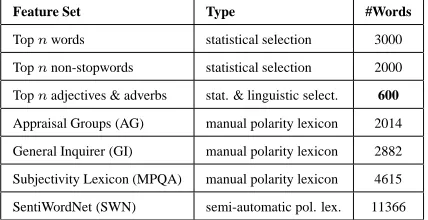
Feature Set Type #Words

Topnwords statistical selection 3000

Topnnon-stopwords statistical selection 2000

Topnadjectives & adverbs stat. & linguistic select. 600

Appraisal Groups (AG) manual polarity lexicon 2014

General Inquirer (GI) manual polarity lexicon 2882

Subjectivity Lexicon (MPQA) manual polarity lexicon 4615

SentiWordNet (SWN) semi-automatic pol. lex. 11366

Table 1: Optimal size of the different feature sets.

but more predictive feature sets are preferable. We use feature sets of frequently occurring adjectives & adverbs in our document collection. The fea-ture sets are extracted using C&C part-of-speech

tagger6. After manually annotating the600 most

frequent stemmed adjectives & adverbs from the movie domain dataset (Pang et al., 2002), we

es-timate that more than20%of the expressions are

ambiguous with regard to part of speech7. Thus,

our selection method if combined with stemming also captures some polar verbs and nouns. By looking at the list of extracted adjectives & ad-verbs from other domains, we observed that unlike current polarity lexicons this method allows both some colloquial expressions, such as crappy, and highly domain-dependent polar expressions, such as creamy or crunchy from the food domain, to be detected.

4.4 Optimal Feature Size

Table 1 lists the optimal size8of the different

fea-ture sets we used in our experiments9. Note that

the subset selection for the polarity lexicons has been explained in Section 4.2. By far, the small-est feature set are adjectives & adverbs; the largsmall-est feature set is SWN.

5 Experiments

The results of all our experiments below are

re-ported on the basis of 20 randomized

partition-ings. Each partitioning comprises a labeled dataset of varying length for training, and another dataset

6_{http://svn.ask.it.usyd.edu.au/trac/} candc

7

e.g. interesting (adj) and interests (noun) are both re-duced to interest

8

The optimal size was determined by testing all semi-supervised algorithms trained on various amounts of labeled documents and1000unlabeled documents.

9_{Due to the stemming we applied some of the entries in}

the original polarity lexicons were conflated.

comprising 1000 documents used as unlabeled

training data and test data10. We also

experi-mented with larger amounts of unlabeled data but did not measure any improvement in performance. The labeled training data and the test data are al-ways mutually exclusive. We report the results of experiments carried out on the movie review database (Pang et al., 2002) (benchmark dataset) and the results of cross-domain experiments us-ing reviews from Rate-It-All. The movie dataset

comprises2000reviews whereas for the other

do-mains we could only acquire1800documents per

domain. All datasets are balanced. We report sta-tistical significance on the basis of a paired t-test

using0.05as the significance level. We only state

the results of the optimally sized feature sets (see Section 4.4). Since there is no difference in per-formance between the optimally sized feature set with the most frequent words and the most fre-quent non-stopwords, we only evaluated the latter

feature set. We used SVMLight11 for SVMs and

TSVMs and SGTLight12for SGT. Feature vectors

consist of tf-idf weighted words appearing in the pre-defined feature set normalized by document length. This produced best results throughout our experiments. Further modifications of the stan-dard configuration of SVMLight (e.g. changing regularization parameters) did not improve per-formance. We also confirm the results from Aue and Gamon (2005) where further modifications

on EM, i.e. by weighting the unlabeled data13,

did not improve performance. For SGTLight we mainly adhered to the standard configuration (as discussed in Joachims (2003)). Since we had no development data for optimizing the only

task-sensitive parameter k we simply took the

opti-mized value for the only text classification cor-pus tested in Joachims (2003) (i.e. Reuters

collec-tion). The current choice (i.e. k = 800) should thus guarantee a fairly unbiased setting. EM is smoothed by absolute discounting (Zhai and Laf-ferty, 2001). All classifiers are run with a reason-able parameter setting but we did not attempt to tune the parameters to the current task. We also stem the entire text since some polarity lexicons we use also include lemmas of inflectional words,

10_{It is not uncommon to use test data as unlabeled}

train-ing data in semi-supervised learntrain-ing (Aue and Gamon, 2005; Joachims, 1999; Joachims, 2003).

11_{http://svmlight.joachims.org} 12

http://sgt.joachims.org

SWN AG GI MPQA GI+Turney

54.20 54.45 59.90 61.95 63.30

Table 2: Accuracy of unsupervised algorithm us-ing different polarity lexicons (movie domain):

best classifier is GI+Turney.

such as nouns and verbs. Moreover, stemming has considerable advantages for the feature set com-prising adjectives & adverbs (see discussion in Section 4.3). In-domain feature sets (i.e. frequent non-stopwords and frequent adjectives & adverbs) are obtained by considering the entire dataset of a particular domain.

5.1 Experiments on the Movie Domain

5.1.1 Unsupervised Algorithms using

Different Polarity Lexicons

Before comparing the different polarity lexicons in the context of semi-supervised learning, we shortly display their performance using a com-pletely unsupervised algorithm. A test document is assigned the polarity with the majority of po-lar expressions in that document. This experiment should give an idea of the intrinsic predictiveness of the polarity lexicons. Table 2 lists the results. Though all lexicons perform significantly better

than the random baseline (i.e. 50%), the best

per-formance of MPQA with61.95is still very low.

We also evaluated an extension GI+Turney

which weights the polar expressions in GI accord-ing to the association scores to a very small num-ber of manually selected highly polar seed words, such as excellent or poor (Turney and Littman,

2003)14. The scores for entries in GI are calculated

in the same way as the scores for words in the web-based lexicon induction method using Pointwise

Mutual Information (Turney, 2002). The

improve-ment is significant, even though the scores have been gained by domain-independent web-data.

In the following, we show that very small amounts of labeled in-domain documents can produce significantly better results using semi-supervised learning.

5.1.2 Comparison of the Different Polarity

Lexicons with Other Feature Sets

Table 3 displays the performance of different clas-sifiers on different feature sets. On average,

polar-14_{Unfortunately, currently only the weights for entries of}

GI were available to us.

ity lexicons perform significantly better than the top 2000 non-stopwords. The same holds for an inexpensive small feature set of in-domain adjec-tives & adverbs. On EM, we achieved even the best performance with the latter feature set. The best performing feature set for the movie dataset is AG. With the exception of EM, it is signifi-cantly better than any other feature set using semi-supervised learning.

5.1.3 Complex Feature Sets that Do Not

Improve Performance

Contrary to our expectations, adding explicit po-larity information to the feature set by including the number of positive and negative polar expres-sions according to the pertaining polarity lexicon did not improve performance. We assume that the meaning of these polar expressions, occasionally even their polarity, varies across different contexts, therefore a unique polarity in the polarity lexicons may not always be correct.

We also experimented with more expressive features by adding bigrams with one token be-ing either a polar expression, an adjective or an adverb. On semi-supervised learning we did not measure any increase in performance. We assume that this is due to data-sparseness. Similar to Ng et al. (2006), we observed an increase in

perfor-mance by approximately2%on supervised

classi-fiers (when more than400 labeled documents are

used).

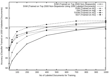
5.1.4 Semi-Supervised Classifiers

We compared all different learning algorithms us-ing their respective best feature sets. Figure 1 dis-plays the results. All semi-supervised algorithms are better than the strict supervised baseline (i.e. SVMs trained on AG) on small amounts of la-beled data. EM gets worse than SVMs trained on

AG when more than 400 labeled documents are

used, but still outperforms SVMs trained on top

2000 non-stopwords when less than 700 labeled

documents are used. TSVMs and SGT, on the other hand, constantly perform better than SVMs. Clearly, the best classifier is SGT which, with the

exception of1000 labeled data, is always

signif-icantly better than any other classifier tested. At

approximately 200 labeled documents, SGT

al-ready performs as well as SVMs trained on a

stan-dard feature set (i.e. top2000non-stopwords)

us-ing1000 labeled documents. The best supervised

pre-20 Labeled Documents 200 Labeled Documents

Top 2000 SWN MPQA GI AG Adj Top 2000 SWN MPQA GI AG Adj

SVM 59.81 61.24 63.07 61.48 62.22 61.44 72.05 74.93 74.35 72.72 75.88 73.14

EM 67.50 67.31 68.73 66.63 69.44 69.54 73.44 76.46 75.02 73.80 75.46 77.32

TSVM 64.57 67.04 66.58 65.53 68.87 68.37 73.48 76.80 75.73 74.72 77.89 75.12

SGT 62.60 67.39 67.10 66.14 70.28 66.58 70.91 77.55 77.78 75.12 80.21 76.90

Table 3: Accuracy of different classifiers on different feature sets using 20 and 200 labeled documents (movie domain): best configuration is SGT+AG.

60 65 70 75 80 85 90

100 200 300 400 500 600 700 800 900 1000

Accuracy (Classifier Trained on 1000 Unlabeled Documents)

No of Labeled Documents for Training

SVM (Trained on Top 2000 Non-Stopwords) SVM (Trained on Top 2000 Non-Stopwords Using 1000 Labeled Documents) SVM (Trained on AG) EM (Trained on Adj) TSVM (Trained on AG) SGT (Trained on AG)

Figure 1: Performance of different learning algo-rithms on the best respective feature set (movie domain): SGT+AG save 800 labeled documents

in comparison to SVM+Top 2000 trained on 1000 labeled documents.

sented in Pang et al. (2002). They report 81.4%

with their most similar configuration using 1400

labeled documents and training on 2633 words.

Just using20labeled documents offers an increase

by 7% in performance in comparison to the best

unsupervised classifier (i.e. GI+Turney displayed in Table 2).

5.2 Cross-Domain Experiments

In order to validate our findings from Section 5.1, we extracted reviews from Rate-It-All. In partic-ular, we want to know whether semi-supervised learning works there as well, whether SGT out-performs other classifiers, whether polarity lex-icons improve performance, and whether adjec-tives and adverbs produce classifiers competitive to average polarity lexicons. We do not attempt to carry out detailed domain studies which would be beyond the scope of this section. We chose four domains from the list of Topic Categories of the website which we thought are very different from

the movie domain and for which we could extract sufficient training data. We took Computer &

In-ternet (computer), Products (products), Sports & Recreation (sports) and Travel, Food, & Culture (travel). We follow the method from Blitzer et al.

(2007) to infer the polarity of the reviews.

Rat-ings with less than3stars are considered negative

reviews whereas ratings with more than 3 stars

are positive reviews. We decided not to consider

mixed reviews, i.e. reviews rated with 3 stars.

In general, we found far fewer mixed reviews15.

On those domains which provided a reasonable amount of data, our initial supervised learning ex-periments showed that mixed polarity can only

be poorly distinguished from definite polarity16.

Manual inspection of a random sample of reviews also showed that a great part of these documents are actually negative reviews. We only extracted

reviews having at least3sentences in order to rule

out too fragmentary instances. We did not filter out mislabeled entries though we are aware of their presence in our set.

Table 4 lists the average performance of all

classifiers on different feature sets using 20

la-beled documents. For the sake of completeness we also include the results from the movie do-main. There is no significant difference among the feature sets using SVMs, but there is a

dif-ference between top2000non-stopwords and the

remaining feature sets on semi-supervised classi-fication (with the exception of EM). All polarity lexicons and adjectives & adverbs perform

signifi-cantly better than top 2000 non-stopwords using

TSVMs and SGT. On average, the performance of EM is significantly worse than any of the other semi-supervised classifiers. The results of TSVMs

15_{In the computer domain, for example, there were only}

approximately200reviews.

16_{A binary classifier trained on900mixed and900definite}

polar reviews from the travel domain only produced an accu-racy of63

.1%on a three fold crossvalidation and the best

are similar with our previous observations on the benchmark dataset. SGT is the best performing classifier (in particular in combination with adjec-tives).

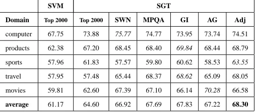
Table 5 shows the performance on the indi-vidual domains and feature sets using 20 labeled documents on SGT. On average, semi-supervised learning improves performance significantly over supervised learning. On some domains (e.g.

com-puter) using a standard feature set (i.e. using top

2000 non-stopwords in the collection) produces

good results. However, in some other domains, such as travel, there is no improvement whatso-ever. Polarity lexicons can perform significantly better than top 2000 non-stopwords (e.g. GI on

travel or, most notably, AG on movie) but there can

also be a domain where they are actually worse than the standard feature set (e.g. the sports do-main). There is no polarity lexicon which consis-tently outperforms all other polarity lexicons on all domains. A feature set comprising in-domain adjectives & adverbs, however, is more robust: Firstly, it never performs worse than the standard

feature set. Secondly, it is never significantly

worse than the average performance of polarity lexicons and, thirdly, there might be some domain, such as sports, where it significantly outperforms any other feature set. Considering the low effort to generate such a feature set should make it particu-larly attractive.

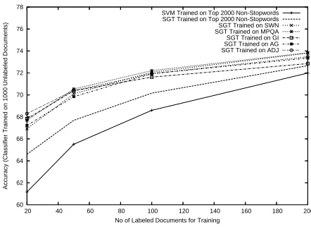
Figure 2 displays the performance of SGT on various feature sets averaged over all domains us-ing various amounts of labeled trainus-ing data. SGT only significantly outperforms SVMs when less

than 200 labeled documents are used.

There-fore, we restricted the figure to the range ending at that size. The lower performance of the av-eraged results must be due to some properties of the Rate-It-All data (either noise or the dataset is more difficult) since the individual performance of the semi-supervised classifiers on the movie do-main was significantly better. Despite the lower performance, we can still use the averaged results to characterize the relation between the different feature sets in semi-supervised learning. Both po-larity lexicons and adjectives & adverbs are sig-nificantly better than top 2000 non-stopwords and there is no significant difference between polarity lexicons and adjectives & adverbs.

All these results support both the competitive-ness of adjective & adverbs and the robustcompetitive-ness

of SGT. Given the best feature set in a particular domain, the average gain in improvement com-pared to SVMs only trained on 20 labeled doc-uments using top 2000 non-stopwords is approx.

8.5%when SGT is used. This is a clear indication

that semi-supervised learning for polarity classi-fication works across all domains when only tiny amounts of labeled data are used.

Top 2000 SWN MPQA GI AG Adj

SVM 61.17 61.13 60.81 61.17 60.77 60.68

EM 64.41 65.09 64.08 63.88 65.10 65.22

TSVM 63.87 66.79 66.51 66.26 65.98 67.20

SGT 64.60 66.92 67.69 67.83 67.22 68.30

Table 4: Average accuracy of different

semi-supervised classifiers across all domains using dif-ferent feature sets (trained on 20 labeled docu-ments & 1000 unlabeled docudocu-ments): best

config-uration is SGT+Adj.

60 62 64 66 68 70 72 74 76 78

20 40 60 80 100 120 140 160 180 200

Accuracy (Classifier Trained on 1000 Unlabeled Documents)

No of Labeled Documents for Training

SVM Trained on Top 2000 Non-Stopwords SGT Trained on Top 2000 Non-Stopwords SGT Trained on SWN SGT Trained on MPQA SGT Trained on GI SGT Trained on AG SGT Trained on ADJ

Figure 2: SGT trained on different amounts of la-beled data and different feature sets averaged over all domains (1000 unlabeled documents):

polar-ity lexicons and Adj are very similar among each other and significantly better than top 2000 non-stopwords.

6 Conclusion

In this paper we have shown that semi-supervised learning can be successfully applied to

document-level polarity classification. Significant

SVM SGT

Domain Top 2000 Top 2000 SWN MPQA GI AG Adj

computer 67.75 73.88 75.77 74.77 73.95 73.74 74.51

products 62.38 67.20 68.45 68.40 69.84 68.44 68.79

sports 57.96 61.83 57.57 59.80 60.62 58.53 63.55

travel 57.95 57.48 65.44 68.37 68.62 65.09 68.05

movies 59.81 62.60 67.39 67.10 66.14 70.28 66.58

average 61.17 64.60 66.92 67.69 67.83 67.22 68.30

Table 5: Accuracy of SGT on different domains using different feature sets (trained on 20 labeled docu-ments & 1000 unlabeled docudocu-ments): on an individual domain either some polarity lexicon or Adj is the

best feature set; on average Adj is the best feature set.

across all amounts of labeled training data. SGT is the classifier which produces significantly bet-ter results than all other semi-supervised classi-fiers used in our experiments. On average, polarity lexicons and adjectives & adverbs perform better than just using frequent in-domain non-stopwords. Adjectives & adverbs are less expensive to obtain and more robust throughout different domains.

Acknowledgements

The authors would like to thank Grzegorz Chrupała, Sab-rina Wilske and Theresa Wilson for interesting discussions. We, in particular, thank Stefan Kazalski for pre-processing the web documents from Rate-It-All. Michael Wiegand was funded by the German research council DFG through the In-ternational Research Training Group between Saarland Uni-versity and UniUni-versity of Edinburgh.

References

A. Aue and M. Gamon. 2005. Customizing Sentiment Classifiers to New Domains: a Case Study. In Proc. of RANLP.

P. Beineke, T. Hastie, and S. Vaithyanathan. 2004. The Sentimental Factor: Improving Review Classifica-tion via Human-Provided InformaClassifica-tion. In Proc. of ACL.

J. Blitzer, M. Dredze, and F. Pereira. 2007. Biogra-phies, Bollywood, Boom-boxes and Blenders:

Do-main Adaptation for Sentiment Classification. In

Proc. of ACL.

A. Esuli and F. Sebastiani. 2006. SentiWordNet:

A Publicly Available Lexical Resource for Opinion Mining. In Proc. of LREC.

M. Gamon. 2004. Sentiment Classification on Cus-tomer Feedback Data: Noisy Data, Large Feature

Vectors, and the Role of Linguistic Analysis. In

Proc. of COLING.

T. Joachims. 1999. Transductive Inference for Text Classification Using Support Vector Machines. In Proc. of ICML.

T. Joachims. 2003. Transductive Learning via Spectral Graph Partitioning. In Proc. of ICML.

A. Kennedy and D. Inkpen. 2005. Sentiment Classifi-cation of Movie Reviews Using Contextual Valence Shifters. In Workshop on the Analysis of Formal and Informal Information Exchang during Negotiations.

V. Ng, S. Dasgupta, and S. M. Niaz Arifin. 2006. Ex-amining the Role of Linguistic Knowledge Sources in the Automatic Identification and Classification of Reviews. In Proc. of ACL.

K. Nigam, A. McCallum, S. Thrun, and T. Mitchell. 2000. Text Classification from Labeled and Unla-beled Documents Using EM. Machine Learning.

B. Pang and L. Lee. 2004. A Sentimental Education: Sentiment Analysis Using Subjectivity Summariza-tion Based on Miminum Cuts. In Proc. of ACL.

B. Pang, L. Lee, and S. Vaithyanathan. 2002. Thumbs up? Sentiment Classification Using Machine Learn-ing Techniques. In Proc. of EMNLP.

F. Salvetti, C. Reichenbach, and S. Lewis. 2006.

Opin-ion Polarity IdentificatOpin-ion of Movie Reviews. In

J. Shanahan, Y. Qu, and J. Wiebe, editors, Comput-ing Attitude and Affect in Text: Theory and Applica-tions. Springer-Verlag.

P. Turney and M. Littman. 2003. Measuring Praise and Criticism: Inference of Semantic Orientation from Association. In Proc. of TOIS.

P. Turney. 2002. Thumbs up or Thumbs down?: Se-mantic Orientation Applied to Unsupervised Classi-fication of Reviews. In Proc. of ACL.

C. Whitelaw, N. Garg, and S. Argamon. 2005. Using Appraisal Groups for Sentiment Analysis. In Proc. of CIKM.

T. Wilson, J. Wiebe, and P. Hoffmann. 2005. Recog-nizing Contextual Polarity in Phrase-level Sentiment Analysis. In Proc. of HLT/EMNLP.

C. Zhai and J. Lafferty. 2001. A Study of Smoothing Methods for Language Models Applied to Informa-tion Retrieval. In Proc. of SIGIR.