Alternative method for testing the unit root null hypothesis in the presence of a break

ALTERNATIVE METHOD FOR TESTING THE UNIT ROOT NULL

HYPOTHESIS IN THE PRESENCE OF A BREAK

by

Seungho Huh and David A Dickey

Department of Statistics, North Carolina State University

Institute of Statistics Mimeograph Series No. 2529

Febniary 200 1

o

ALTERNATIVE ME1lJOD FUR TESTING 1UE UNIT ROO!' NUlL HYl'Ol'HESIS IN 1UE PRESmCE OF A BREAK

BY

SE1JNGID HUH AND DAVID A DIa<EY

-DEPT. OF Sl'ATISfICS, NCSU

MIMED 00•• 2529. Feb. 2001

Presence of a Break

Seungho Huh and David A. Dickey

Department of Statistics, North Carolina State University, Raleigh, NC27695-8203,

•

Abstract In this paper, we suggest alternative test statistics for testing the unit

root null hypothesis in the presence of a trend-break. Our new test procedure which

we call the "bisection" method is based on the idea of subgrouping. The idea here is

to split the data in half and look at the minimum of the resulting two unit root test

statistics. This avoids the necessity of searching for the break. It uses all the data in

the sense that the minimum is chosen, but clearly is not efficient in its use of the data.

We anticipate paying a price in power for a gain in simplicity. Considering some data

generating processes, we display empirical size and power results from simulation. We

also apply our bisection method to the well-known Nelson and Plosser (1982) data set

and compare the results with those of other researchers. The simple bisection method

rejects unit roots in several, but not all, of the series for which the more complicated

search methods reject.

1

Introduction

Since the pioneering work by Perron (1989), many researchers have been interested

in testing for a unit root in time series with a trend-break. It is known that power

decreases in finite samples as the trend-break becomes larger when the usual

Dickey-Fuller (1979) test is used.

Perron (1989) suggested formal statistical tests of the null hypothesis of a unit

root which can distinguish the unit root hypothesis from that of stationarity around

a trend with a single trend-break (either in the intercept or the slope). His original

approach assumed the trend-break is known a priori and treated as exogenous. Perron

(1997) and Vogelsang and Perron (1998), on the other hand, considered unit root tests

treating the date of a possible trend-break as unknown. They introduced various

methods of choosing the break date. A variation of Perron's (1989) test in which the

break point is estimated rather than fixed was also studied by Zivot and Andrews

•

the break time is unknown, it is ignored rather than estimated. Using the new test

statistic, we perform a Monte Carlo simulation to obtain its empirical powers which

are rather invariant to the break size.

Section 2 describes the idea of subgrouping and simulation results to find the

optimal number of subgroups. As a result, we suggest new test statistics in section

3. Section 4 presents the data generating processes and some empirical power results

from a Monte Carlo simulation. In section 5, we apply our test procedure to the real

data analyzed originally by Nelson and Plosser (1982). We finally make concluding

remarks in section 6.

2

Subgrouping of data

Our new test procedure is based on the idea of dividing the whole data into some

subgroups of the same size. For each subgroup, a certaint type statistic is calculated.

Then the minimum of all these statistics is defined as a new test statistic for the unit

root null hypothesis in time series with a break.

Suppose we have stationary series around a broken trend. After dividing the

data into subgroups, we expect to have a smaller value of the test statistic from a

subgroup without a break than from another subgroup with a break. Therefore taking

the minimum among all the statistics might give us reasonable power as we are using

left tailed tests. This is a key motivation for our subgrouping idea.

The approach by Perron (1989) assumes the break point is known a priori. Using

dummy variables, he combines the data before the break with the data after the

break. We do not have to assume a known break point in our new procedure.

With the break point assumed unknown, Zivot and Andrews (1992) choose the

Then they take thet type statistic giving that break point. Our procedure is simpler

because it does not consider estimating the unknown break point.

We perform some simulations to decide the optimal number of subgroups. The

data generating process given by (1) in section 4 is used for various numbers of

subgroups. We consider

nCo-l)

type statistics from the ordinary least squares (OL8) estimator, the simple symmetric (88) estimator and the weighted symmetric (W8)

estimator. The number of replications is 5,000 and the sample size per replication is

n

=

100. We consider the break point c

=

36 (for OL8) or c

=

37 (for 88 and W8)

and the break size () = 1, 3, 5 and 7. In Tables 1 - 3 and Figures 1 - 3, we show

empirical size and power results from simulation.

Clearly the optimal number of subgroups is 2. We expect similar results for t

type statistics. The next section describes our new test procedure which we call the

"bisection" method.

3

Bisection method

From the previous work by Leybourne et al (1998) and Huh and Dickey (1999), we

know that, in the presence of an early break, the conventional Dickey-Fuller (1979)

test based on the least squares estimator can be subject to serious size distortion

but tests based on the weighted symmetric estimator cure this problem. Therefore

our bisection method in this paper is based on the W8 estimator of p,

Pw,

and the

associated pivotal statistic Tw in the non-zero mean AR(1) process

Our new bisection test statistic is defined as

where Tw,k is _Tw for subgroup k for k = 1,2. Each subgroup is supposed to have

•

process (1) in section 4. We assume n

=

100, c

=

75, 0

=

5 and p

=

.7. Notice that

the empirical distributions ofTw,l and T~ are very close to each other since the break

is in the second subgroup (c = 75). That does not necessarily mean that they have

the same power for a certain p because the critical values are different as shown in

Figure 4. In the figure, the vertical line on the left denotes the critical value forT~, so

the power for T~ is lower than that for Tw,l as can be seen in Figure 5. This generally

holds good for other values ofp.

As to the linear trend adjusted case, we consider the WS estimator ofp and the

associated pivotal statistic TW,T in the model

rt

= J1

+

f3t

+

Prt-l

+

et·

TW,T can be regarded as the linear trend adjusted version ofTw . We then use T~,T' the

minimum of two TW,T statistics, as a new test statistic. See Huh and Dickey (1999)

for more details about Tw and Tw,T"

4

Empirical size and power results

In this section, we display some size and power simulation results using bisection

test statistics.

We consider two data generating processes (DGPs) given by

rt

rt

OaI(t>

c)

+

_{W t , Wt} = _pWt-1

+

et, t = 1,2, ,n

'Ya(t - c)I(t

>

c)

+

W t , Wt

=

pWt-1

+

et, t

=

1,2, ,n

(1)

(2)

where the et are normal independent (0,a2

) random variables and c is the break point.

We can assume a

=

1 since

Pw

is the ratio of two quadratic forms so it is invariant to

,

and DGP (2) to a break-in-slope model with slopes 0 and

'Ya.

Figures 6 - 9 present

some typical time series data generated from DGPs (1) and (2).

We perform a Monte Carlo simulation for some values of 0, "I, c and p. The

number of replications is 5,000 and the sample size per replication is n = 100. The

critical values for T~ and T~,T are also calculated by simulation.

4.1

Data with a break in level

4.1.1 Mean adjusted case

For DGP (1), we first use the mean adjusted statistics T_w and T~. As might be

expected from the results in Huh and Dickey (1999), neither Tw nor T~ show size

distortion for DGP (1).

Ifwe use T~ as a test statistic, the powers are in general higher than those for the

usualTw when there is a break. Some exceptions are for the early break (c= 1) or the

late break (c = 99). For given p, the powers for T~ are relatively invariant whereas

those for the usual Tw decrease dramatically as 0 becomes larger.

Ifthere is no break (0 = 0), on the other hand, the usualTw is more powerful than

T~. This is so especially for large values ofp. Notice that our power results for T w in

Table 4 agree closely with those of Pantula et al (1994).

Table 4 and Figures 10 - 12 present the empirical size and power results for DGP

(1) using Tw and T~. As might be expected, Tw outperforms T~ for small breaks and

T~ outperforms Tw for larger breaks. In all cases, T~ is more uniform with respect to

A.

We compare the size and power properties of our test procedure with those of

Vogelsang and Perron (1998). They consider a DGP

Yt

OI(t

> Tb)

+

'Y(t - Tb)I(t

> Tt)

+

Zt,

•

(Tb(t&), n(!ti'l), Tb(ti') and n(FO,i')) according to the methods of estimating the true

break date. For their simulation, n

=

100 and Tt

=

50. When p

=

.8, our T~ shows

higher power than most of their statistics regardless of the break size (). Although one

statistic (n(t&)) with ()= 10 has higher power than our T~, that can be attributed to

its size distortion problem. In Table 5, we show empirical powers for DGP (1) using

various statistics.

4.1.2 Linear trend adjusted case

We next use the linear trend adjusted statistics TW,T and T~,T for DGP (1). Both

TW,T and T~,T retain empirical sizes (p = 1) close to the nominal 5% significance level.

When there is no break, TW,T shows higher power than T~,T for given p. Notice

also that TW,T and T~,T generate lower power than Tw and T~ respectively.

When the break is fairly big (()

=

10), the powers for T~_,T are generally higher

than those for TW,T' As in the mean adjusted case, the powers for T~,T are relatively

invariant compared with those for TW,T'

The empirical size and power results using TW,T and T~,T are presented in Table 6

and Figures 13 - 15.

4.2

Data with a break in slope

For DGP (2) which represents a break-in-slope model, we adopt the linear trend

adjusted statistics TW,T and T~,T' Even though both TW,T and T~,T retain the nominal

5% significance level, TW,T becomes severely under-sized as I grows larger.

As expected, T~,Tgives smaller powers thanTW,T if there is no break. AsI becomes larger, the powers for TW,T decrease dramatically except for the early or late breaks

whereas T~,T maintains reasonable powers. T~,T is generally more powerful than TW,T

•

The simulation results for DGP (2) using IW,T and I~,T are displayed in Table 7

and Figures 16 - 18.

To compare with the results of Vogelsang and Perron (1998), we consider DGP

(3) with a

=

'l/J

= () =

0 which is exactly the same as our DGP (2). When p

=

.8, the

powers of our I~_,T are as good as those of their statistics for some values of'Y. Power

comparisons between I~,Tand statistics of Vogelsang and Perron (1998) are displayed

in Table 8.

5

Empirical applications

We now apply our bisection method to the data set analyzed originally by Nelson

and Plosser (1982). The data set consists of 14 major macroeconomic time series

which include measures of output, spending, money, prices and interest rates. The

data are annual, generally averages for the year, with starting dates from 1860 to

1909 and ending in 1970 in all cases. We analyze the natural logarithm of all the data

except for the interest rate series, which is analyzed in levels form. Many researchers

have referred to this data set. See Nelson and Plosser (1982) for more details about

the data set.

In Table 9, we compare our unit root test results with those of Nelson and Plosser

(1982), Perron (1989), Zivot and Andrews (1992) and Perron (1997). Numbers are

the values of the test statistics.

Nelson and Plosser (1982) apply the usual Dickey-Fuller test with extra lags of

the first differences of the data (augmented Dickey-Fuller test). Methods of Perron

(1989) and Zivot and Andrews (1992) are briefly described in section 2. Perron

(1997) is closely related to and complements Zivot and Andrews (1992) in that similar

procedures are analyzed. See the original articles for more details.

Our method adopts the number of augmenting terms, k, producing the minimum

..

erated from simulation. Our bisection method using T~,T rejects the unit root null

hypothesis at a = .05 for the series "Real GNP", "Real per capita GNP", "Industrial

production", "Unemployment rate", "Real wages" and "Money stock".

6

Summary

In this work, we suggest new test statistics T~ and T~,T for testing the unit root

null hypothesis in the presence of a trend break. These statistics are based on the

idea of dividing the data into subgroups of the same size. The optimal number of

subgroups turns out to be 2.

Our bisection method can be used without assuming a known break point unlike

Perron's (1989) original approach. It is simpler than the methods of Zivot and An-drews (1992) and Perron (1997). When there is a trend-break and the break size is

fairly big, the empirical powers of the new statistics are in general higher than the

usual T w and TW,T respectively. Based on simulation studies, the power properties of

our test procedure are as good as those of Vogelsang and Perron's (1998).

We also apply our procedure to the well-known Nelson and Plosser (1982) data

•

Table 1: Empirical size and power for DGP (1) using various subgroups (OLS, n = 100, C

=

36)

No. of subgroups 1 2 5 10 20

() =

1, P =.1 1.0000 1.0000 0.9994 0.6938 0.0994

.2 1.0000 1.0000 0.9936 0.5424 0.0884

.3 1.0000 1.0000 0.9600 0.4026 0.0826

.4 1.0000 1.0000 0.8554 0.2948 0.0752

.5 1.0000 0.9984 0.6788 0.2096 0.0682

.6 1.0000 0.9780 0.4740 0.1434 0.0634

.7 0.9974 0.8388 0.2898 0.0974 0.0598

.8 0.9132 0.5042 0.1626 0.0744 0.0544

.9 0.4288 0.1870 0.0962 0.0528 0.0524

1 0.0474 0.0470 0.0530 0.0504 0.0488

() =

3, p=.1 1.0000 1.0000 0.9986 0.6764 0.0946

.2 1.0000 1.0000 0.9888 0.5246 0.0848

.3 0.9996 1.0000 0.9416 0.3856 0.0798

.4 0.9976 0.9992 0.8126 0.2806 0.0728

.5 0.9806 0.9852 0.6260 0.1980 0.0658

.6 0.9144 0.9052 0.4298 0.1342 0.0606

.7 0.7458 0.6786 0.2564 0.0930 0.0576

.8 0.4824 0.3650 0.1472 0.0710 0.0530

.9 0.2382 0.1464 0.0886 0.0476 0.0504

No. of subgroups 1 2 5 10 20

() =

5, p =.1 0.7650 1.0000 0.9986 0.6760 0.0946

.2 0.5990 1.0000 0.9886 0.5240 0.0844

.3 0.4212 1.0000 0.9408 0.3846 0.0792

.4 0.2654 0.9990 0.8104 0.2792 0.0726

.5 0.1612 0.9818 0.6224 0.1966 0.0656

.6 0.0976 0.8920 0.4230 0.1330 0.0604

.7 0.0712 0.6440 0.2482 0.0908 0.0576

.8 0.0626 0.3116 0.1394 0.0694 0.0530

.9 0.0686 0.1114 0.0808 0.0466 0.0504

1 0.0386 0.0418 0.0464 0.0470 0.0476

() =

7, p =.1 0.0064 1.0000 0.9986 0.6760 0.0946

.2 0.0018 1.0000 0.9886 0.5240 0.0900

.3 0.0004 1.0000 0.9408 0.3846 0.0768

.4 0 0.9990 0.8104 0.2792 0.0724

.5 0 0.9818 0.6224 0.1966 0.0708

.6 0 0.8920 0.4230 0.1330 0.0678

.7 0.0004 0.6424 0.2480 0.0908 0.0632

.8 0.0008 0.3060 0.1382 0.0692 0.0504

.9 0.0128 0.0978 0.0790 0.0464 0.0546

Table 2: Empirical size and power for DGP (1) using various subgroups (88, n

=

100, c

=

37)

No. of subgroups 1 2 5 10 20

() =

1, P =.1 1.0000 1.0000 0.9968 0.6278 0.1916

.2 1.0000 1.0000 0.9806 0.4670 0.1602

.3 1.0000 1.0000 0.9178 0.3584 0.1266

.4 1.0000 0.9998 0.7978 0.2696 0.1144

.5 1.0000 0.9992 0.5980 0.1874 0.1058

.6 1.0000 0.9754 0.3856 0.1336 0.0802

.7 0.9982 0.8314 0.2360 0.1024 0.0766

.8 0.9384 0.4970 0.1326 0.0730 0.0698

.9 0.4960 0.1856 0.0800 0.0644 0.0542

1 0.0536 0.0470 0.0512 0.0482 0.0494

() =

3, P =.1 1.0000 1.0000 0.9934 0.6062 0.1872

.2 1.0000 1.0000 0.9684 0.4490 0.1562

.3 0.9998 1.0000 0.8896 0.3418 0.1242

.4 0.9980 0.9990 0.7462 0.2516 0.1106

.5 0.9866 0.9886 0.5396 0.1736 0.1010

.6 0.9324 0.9036 0.3392 0.1258 0.0778

.7 0.7828 0.6590 0.2152 0.0946 0.0732

.8 0.5340 0.3600 0.1242 0.0682 0.0682

.9 0.2770 0.1548 0.0734 0.0600 0.0522

No. of subgroups 1 2 5 10 20

() =

5, p=.1 0.8080 1.0000 0.9932 0.6060 0.1854

.2 0.6590 1.0000 0.9682 0.4482 0.1544

.3 0.4718 1.0000 0.8888 0.3416 0.1224

.4 0.3176 0.9986 0.7420 0.2510 0.1092

.5 0.1868 0.9848 0.5340 0.1724 0.1002

.6 0.1244 0.8860 0.3294 0.1246 0.0770

.7 0.0832 0.6200 0.2018 0.0930 0.0722

.8 0.0680 0.3078 0.1142 0.0666 0.0672

.9 0.0804 0.1162 0.0672 0.0586 0.0506

1 0.0436 0.0406 0.0448 0.0444 0.0474

() =

7, p=.1 0.0110 1.0000 0.9932 0.6060 0.1852

.2 0.0024 1.0000 0.9682 0.4482 0.1544

.3 0.0014 1.0000 0.8888 0.3416 0.1224

.4 0 0.9986 0.7420 0.2510 0.1092

.5 0 0.9848 0.5338 0.1724 0.1002

.6 0.0002 0.8860 0.3292 0.1246 0.0768

.7 0 0.6184 0.2004 0.0930 0.0722

.8 0.0014 0.3012 0.1132 0.0666 0.0672

.9 0.0154 0.1008 0.0654 0.0584 0.0504

Table 3: Empirical size and power for DGP (1) using various subgroups (WS, n = 100, c

=

37)

No. of subgroups 1 2 5 10 20

() =

1, p=.1 1.0000 1.0000 0.9988 0.5346 0.1500

.2 1.0000 1.0000 0.9842 0.4218 0.1246

.3 1.0000 1.0000 0.9312 0.3052 0.1012

.4 1.0000 0.9998 0.8060 0.2262 0.0958

.5 1.0000 0.9992 0.6092 0.1666 0.0904

.6 1.0000 0.9844 0.4166 0.1218 0.0698

.7 0.9992 0.8750 0.2438 0.0932 0.0634

.8 0.9592 0.5470 0.1486 0.0708 0.0600

.9 0.5518 0.1942 0.0738 0.0560 0.0498

1 0.0526 0.0488 0.0514 0.0484 0.0484

() =

3, P =.1 1.0000 1.0000 0.9966 0.5144 0.1456

.2 1.0000 1.0000 0.9748 0.4044 0.1204

.3 0.9996 1.0000 0.9050 0.2880 0.0996

.4 0.9994 0.9992 0.7600 0.2122 0.0928

.5 0.9924 0.9914 0.5554 0.1562 0.0866

.6 0.9576 0.9318 0.3722 0.1148 0.0678

.7 0.8338 0.7214 0.2154 0.0882 0.0622

.8 0.5912 0.4088 0.1344 0.0658 0.0590

.9 0.3070 0.1544 0.0688 0.0522 0.0468

No. of subgroups 1 2 5 10 20

() =

5, p =.1 0.8564 1.0000 0.9966 0.5142 0.1432

.2 0.7314 1.0000 0.9746 0.4042 0.1182

.3 0.5670 0.9998 0.9014 0.2872 0.0964

.4 0.4028 0.9978 0.7582 0.2118 0.0904

.5 0.2524 0.9874 0.5490 0.1556 0.0844

.6 0.1656 0.9174 0.3654 0.1144 0.0664

.7 0.1088 0.6748 0.2084 0.0872 0.0610

.8 0.0846 0.3446 0.1248 0.0640 0.0574

.9 0.0876 0.1172 0.0630 0.0512 0.0462

1 0.0452 0.0410 0.0452 0.0446 0.0466

() =

7, p =.1 0.0232 1.0000 0.9966 0.5142 0.1428

.2 0.0064 1.0000 0.9746 0.4042 0.1178

.3 0.0020 0.9998 0.9014 0.2872 0.0962

.4 0.0004 0.9978 0.7582 0.2118 0.0906

.5 0 0.9874 0.5490 0.1556 0.0842

.6 0.0002 0.9172 0.3648 0.1144 0.0662

.7 0.0002 0.6736 0.2076 0.0872 0.0604

.8 0.0016 0.3366 0.1240 0.0640 0.0570

.9 0.0142 0.1024 0.0612 0.0512 0.0460

Table 4: Empirical size and power for DGP (1) using Tw and T~

(}=o (}=5 () = 10

p C _Tw T*_{w Tw} T*_{w Tw} T*_w

0.5 1 1.0000 1.0000 0.9998 0.9968 0.9810 0.9900

0.5 20 1.0000 1.0000 0.6532 0.9878 0.0000 0.9884

0.5 50 1.0000 1.0000 0.1898 1.0000 0.0000 0.9996

0.5 80 1.0000 0.9996 0.6576 0.9884 0.0000 0.9902

0.5 99 1.0000 0.9996 1.0000 0.9970 0.9774 0.9940

0.8 1 0.9834 0.6006 0.8782 0.4746 0.5392 0.3858

0.8 20 0.9824 0.5890 0.2132 0.3476 0.0000 0.3416

0.8 50 0.9854 0.5994 0.0780 0.5918 0.0000 0.5960

0.8 80 0.9840 0.6020 0.2594 0.4016 0.0000 0.4056

0.8 99 0.9816 0.5918 0.8532 0.5094 0.5614 0.4784

0.9 1 0.6090 0.2256 0.4218 0.1690 0.1904 0.1362

0.9 20 0.6236 0.2244 0.1214 0.1210 0.0006 0.0952

0.9 50 0.6220 0.2316 0.0912 0.2332 0.0002 0.2234

0.9 80 0.6294 0.2188 0.1746 0.1496 0.0056 0.1380

0.9 99 0.6256 0.2258 0.4632 0.2020 0.2708 0.1790

1 1 0.0588 0.0516 0.0504 0.0494 0.0480 0.0502

1 20 0.0538 0.0524 0.0470 0.0398 0.0358 0.0298

1 50 0.0516 0.0496 0.0518 0.0484 0.0328 0.0498

1 80 0.0508 0.0466 0.0496 0.0434 0.0404 0.0310

P 1 0.8

() _{0 5 10 0 5 10}

n(t&)t

0.040 0.108 0.507 0.295 0.435 0.861

n(lt-yl)t

0.049 0.048 0.032 0.301 0.098 0.042

Tb(t-y)

t 0.050 0.050 0.040 0.350 0.133 0.055

n(F' ,

_(),'Y)t 0.052 0.050 0.020 0.339 0.194 0.163

r*_w 0.050 0.048 0.050 0.599 0.592 0.596

Table 6: Empirical size and power for DGP (1) using TW,T and T:U,T

0=0 0=5 0=10

P c TW,T T:U T TW,T T WT* TW,T T:U T

0.5 1 1.0000 0.9880 0.9986 0.9498 0.9270 0.9088

0.5 20 1.0000 0.9848 0.8418 0.8906 0.0018 0.8802

0.5 50 1.0000 0.9850 0.9720 0.9850 0.0992 0.9854

0.5 80 1.0000 0.9844 0.8406 0.9044 0.0012 0.8854

0.5 99 1.0000 0.9892 0.9984 0.9516 0.9258 0.9170

0.8 1 0.8292 0.2970 0.6226 0.2494 0.3082 0.1912

0.8 20 0.8386 0.2954 0.2842 0.2016 0.0050 0.1486

0.8 50 0.8346 0.3040 0.4354 0.3068 0.0484 0.3016

0.8 80 0.8312 0.2986 0.2946 0.2152 0.0060 0.1848

0.8 99 0.8238 0.2938 0.6160 0.2542 0.3454 0.2372

0.9 1 0.3066 0.1084 0.2150 0.0936 0.0982 0.0816

0.9 20 0.2968 0.1126 0.1298 0.0932 0.0162 0.0594

0.9 50 0.2974 0.1152 0.1874 0.1130 0.0528 0.1090

0.9 80 0.2906 0.1108 0.1426 0.0936 0.0232 0.0654

0.9 99 0.2982 0.1082 0.2306 0.1048 0.1318 0.0902

1 1 0.0574 0.0558 0.0544 0.0524 0.0426 0.0458

1 20 0.0620 0.0496 0.0496 0.0470 0.0342 0.0316

1 50 0.0540 0.0498 0.0528 0.0466 0.0342 0.0480

1 80 0.0498 0.0502 0.0536 0.0448 0.0362 0.0314

"(=0 "(=1 "(=2

P c TW,T T* * TW,T *

WT TW,T TWT TWT

0.5 1 1.0000 0.9858 1.0000 0.9872 1.0000 0.9860

0.5 20 1.0000 0.9862 0.0000 0.8884 0.0000 0.8804

0.5 50 1.0000 0.9860 0.0000 0.9852 0.0000 0.9892

0.5 80 1.0000 0.9862 0.0000 0.8848 0.0000 0.8852

0.5 99 1.0000 0.9868 1.0000 0.9860 1.0000 0.9822

0.8 1 0.8296 0.3098 0.8172 0.2974 0.8322 0.3084

0.8 20 0.8170 0.2934 0.0000 0.1544 0.0000 0.1572

0.8 50 0.8256 0.3060 0.0000 0.2980 0.0000 0.3020

0.8 80 0.8330 0.3126 0.0000 0.1704 0.0000 0.1672

0.8 99 0.8170 0.3016 0.8138 0.2940 0.7774 0.3064

0.9 1 0.2962 0.1128 0.2994 0.1006 0.3002 0.1088

0.9 20 0.3050 0.1138 0.0000 0.0524 0.0000 0.0538

0.9 50 0.2968 0.1106 0.0000 0.1118 0.0000 0.1206

0.9 80 0.2974 0.1078 0.0000 0.0624 0.0000 0.0582

0.9 99 0.3026 0.1130 0.2894 0.1114 0.0552 0.1180

1 1 0.0572 0.0510 0.0556 0.0568 0.0566 0.0470

1 20 0.0526 0.0498 0.0000 0.0302 0.0000 0.0282

1 50 0.0552 0.0504 0.0000 0.0496 0.0000 0.0516

1 80 0.0622 0.0514 0.0000 0.0260 0.0000 0.0270

Table 8: Empirical size and power for DGP (2) using various statistics (n = 100, c= 50)

p 1 0.8

'Y 0 1 2 0 1 2

Tb(ta)t

0.040 0.044 0.076 0.295 0.236 0.386

n(lt-yl)t 0.049 0.036 0.032 0.301 0.239 0.230

n(t-y)t

0.050 0.072 0.061 0.350 0.376 0.371

n(F-

_(),'YA)t 0.052 0.027 0.021 0.339 0.193 0.184

T~r 0.050 0.050 0.052 0.306 0.298 0.302

Series n N&pt P1§ _Z&A' P21l Bisection**

Real GNP 62 -2.99 -5.03* -5.58* -5.93* -4.09t

Nominal GNP 62 -2.32 -5.42* -5.82* -8.16* -2.28

Real per capita GNP 62 -3.04 -4.09t -4.61 -4.81 -3.71t

Industrial production 111 -2.53 -5.47* -5.95* -6.01* -5.72t

Employment 81 -2.66 -4.51* -4.95t -5.14t -3.46

Unemployment rate 81 -3.55t N/A N/A N/A -4.06t

GNP deflator 82 -2.52 -4.04t -4.12 -4.14 -2.67

Consumer prices 111 -1.97 -1.28 -2.76 -3.09 -3.18

Wages 71 -2.09 -5.41* -5.30t -5.41t -2.93

Real wages 71 -3.04 -4.28t -4.74 -5.41 -4.35t

Money stock 82 -3.08 -4.29t -4.34 -4.69 -4.48t

Velocity 102 -1.66 -1.66 -3.39 -2.81 -2.44

Interest rate 71 0.686 -0.45 -0.98 -1.35 -0.80

Common stock prices 100 -2.05 -4.87t -5.61* -5.50t -3.34

*statistical significance at the 1%level

tstatistical significance at the 5% level lNelson and Plosser (1982)

§Perron (1989)

'Zivot and Andrews (1992) IIPerron (1997)

theta=1 theta=3 \ \ \ \ \ \ \ \ \ \ ,,_, , ,_, , ,_{, ,} C?

....

IX)

a

"- <0 Q)

a

:= 0 a.. "'<t

a

C\I

a

---

_{---..:=:..-...:.:.}

--

...'. C? IX)

a

Qj <0

a

:= 0 a.. "'<t

a

C\I

a

\ \ \ \ \ \ \ \ \ ,, ,, ,, , ,_, , ,

---

... . .

0.2 0.4 0.6 0.8 1.0

rho

0.2 0.4 0.6 0.8 1.0

rho

theta=5 theta=7

C? C?

IX) IX)

0

a

\ \

<0 \ _<0 \

L-a

\

"-a

\

Q) , Q) \

:=

,,

:=

\

\

0 \ 0 \

a.. _"'<t \ a..

~ \ \ \

a

\ 0 , ,_, ,_, ,_, ,_, , C\I ,

C\I , ,

a

,,_,

a

,,_,

, ,

---

---~.:..~

---

-0

a

0.2 0.4 0.6 0.8 1.0 0.2 0.4 0.6 0.8 1.0

rho rho

C! C!

..

co co

c:i c:i

...

co \ co

Q) c:i \ Q; _c:i

~ \

~

\

0 \ 0

a.. \ a..

"<t \ _"<t

c:i \

c:i

\

..

..

..

..

C\J

..

..

C\J

c:i ..._...

..

..

..

_c:i

'.

...

----

..

'.

-.:.~~..-..

0.2 0.4 0.6 0.8 1.0

rho

theta

=

5

... \ \ \ \ \ \_.. \_.. ..

..

..

..

..

'"""---... "... . .

---0.2 0.4 0.6 0.8 1.0

rho

theta

=

7

..._... ...

---C! co c:i

...

co Q) c:i ~ 0 a.. -.:J: a C\J c:i \ \ \ \ \ .._.. \_..

..

..

.. ..

_..

....

0.2 0.4 0.6 0.8 1.0

rho C! co c:i

...

co Q) c:i ~ 0 a.. _"<t c:i C\J c:i a c:i ... \ \ \ \ \ .._.. \_..

..

.. .._..

..

..

... ...

---0.2 0.4 0.6 0.8 1.0

rho

C! co 0

...

CD Q) 0 :;: 0 a.. '<:I: a C\I 0 C! co 0 CD Qi 0 :;: 0 a.. _~ 0 C\I 0

theta= 1

\ \ \ \ \ \ \ \ , ,_, , " .

--.::.~::-.:.~-0.2 0.4 0.6 0.8 1.0

rho

theta=5

.... '. \ \ \ \ \ \ \ \_, , ,_,

--

... ...

- - - - -..:

:--..:::.2::.:.:~

0.2 0.4 0.6 0.8 1.0

rho C! co 0

...

CD Q) 0 :;: 0 a.. _~ 0 C\I 0 C! co 0

...

CD Q) 0 :;: 0 a.. _~ 0 C\I 0 a 0

theta=3

... ,, ,, ,,_, \ , ,_, , , '.

-

-

- - --..:::.'::~...

0.2 0.4 0.6 0.8 1.0

rho

theta=7

... \ \ \ \ \ \ \ \ , ,_, --"':~-..:::.2:~.

0.2 0.4 0.6 0.8 1.0

rho

-4 -3 -2 -1 0 1

test statistics

Taul R: R: R: Tau2 '.n

"T .rr. _Tau

J. Taul Tau2 Tau

: /"\

, : \

·1

ri.

! I 1\

I \

: f \

if

\

'{ i

[ \

I '

\

J

']

,l"E;:

\

/.~

\",,;.

~ \

M V

;

,

; ,,;~

'M 'I

l ' /

I

;~{

1

/

r

[1mHH Taum Taum

Legend f(x) 130 120 110 100 90 80 70 60 50 40 30 20 10 0

-7 -6 -5

0.5

Legend

0.6

'T'--'''' -"F Tau

L'- n

I I

0.7 0.8

rho

M ~1- M Taum Taul

0.9

R R R Tau2

1.0

Figure 5: Empirical size and power of test statistics (WS, n = 100, C= 75 and () = 5;

>-C\I

o

>-C\I

o

o

20 40 60 80 100

o

20 40 60 80 100

theta

=

5 theta= 10

0

<D

CO

'<t _<D

>- C\I >- '<t

C\I

0

0

~ _~

0 20 40 60 80 100 0 20 40 60 80 100

theta= 0 theta= 2.5

0 0

u;>

>-

>-LO

0

-r;-0

LO

....

,

0 20 40 60 80 100 0 20 40 60 80 100

theta= 5 theta= 10

>-o

C\I

LO

o

LO

o

>- 0

o 20 40 60 80 100 o 20 40 60 80 100

>-o

'<t

I

In

~

M

.r

,

H

"

I~

~

~

v

o

20 40 60 80 100

gamma=1

>-o

C\l

o

LO

o

o

20 40 60 80 100

gamma=2

0

LO

0

'<t

0

C')

>-0

C\l

0

0

0 20 40 60 80 100

0 0

...

0

lX)

0

CD

>-0

'<t

0

C\l

0

0 20 40 60 80 100

gamma=0

0

C")

0

....

LO

C\l

0

C\l

>- LO

>-LO

0 ..-0

LO

o

20 40 60 80 100

gamma=0.5

o

20 40 60 80 100

gamma= 1

0

LO

0

~

0

C")

>- 0

C\l

0

0

o

20 40 60 80 100

gamma=2

0 0

0

co

0

CD

>-0

~

0

C\l

0

0 20 40 60 80 100

~ Q) ~ o a.. to en en c:i o en en c:i \.j [""

j .

en c:i to c:i ~ Q) f'o.. ~ _c:i 0 a.. <0 c:i ~ 0

0.0 0.4 0.8 0.0 0.4 0.8

Lambda Lambda

rho=O.9 rho=1

0.8 0.4

/\/\\\

j

'i

\\i

I

0.0 LO LO 0 c:i Q> ~ 0 0 LO a.. 0 c:i LO '<t 0 c:i ...·f 0.8 ... 0.4 LO c:i ~ '<t Q) c:i ~ 0 a.. M c:i C\I c:i .. 0.0 Lambda Lambda

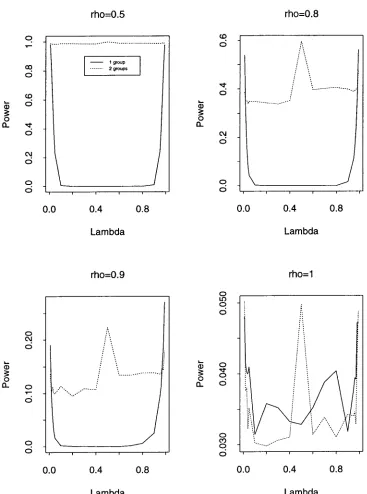
Figure 10: Empirical size and power for DGP (1) using

T

w (1 group) and

T:V

(2 groups)

rho=0.5 rho=0.8

q _{1 group}

CO 2groups

0

CO

0

CD

0

CD _CD CD

/

...

~ ₀ ~

0 0

a.. a.. "d:

0 "d:

0

C\l

0

C\l

0

0.0 0.4 0.8 0.0 0.4 0.8

Lambda Lambda

rho=0.9 rho=1

CD

~

o

a..

C\l

o

". . / '..

...

...

Q)

~ o

a..

o

1O

o

o

o

'<t

o

o

0.0 0.4 0.8 0.0 0.4 0.8

Lambda Lambda

~ ,.... ~ 0 co

...

0 Q) 3: 0 a- '<t 0 C\J 0 0 0 ...----_ -- .

r-

19roup

I

I 2groups

(fi 3: o a-C\J

o

o

o

1\

.~-- - . ~'...' 0.0 0.4 Lambda

0.8 0.0 0.4

Lambda 0.8 rho=O.9 rho=1 0 LO ~ 0 , 0 _!\

C\J _:...

0

j

\m

...

...

₀

Q) Q)

3: 3: '<t0

0 0

0

a- 0 _':....

a-0

0

1\

0 C') ' "

0 ~₀

0.0 0.4 0.8 0.0 0.4 0.8

Lambda Lambda

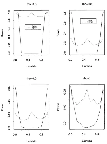
Figure 12: Empirical size and power for DGP (1) usingTw (1 group) andT~ (2 groups)

rho=O.5 rho=0.8 ... .... Q) ~ o a.. o q to (J)

o

/... / . ....: ... \...: \1 \./ 'oJ :: I"'-0 CD 0 .... Q) ~ I() 0 ₀ a.. '<t 0 C') 0 ".:,.,

f=

1group

1

2groups

...;

0.0 0.4

Lambda

0.8 0.0 0.4

Lambda 0.8 rho=O.9 rho=1

~

to I() I() 0 N 0 0 '<t I() 0 0

.... N .... ₀

Q)

0 Q)

~ ~

0 0

a.. a.. ₀

I() I()

0

0 0

0 i .. · .. · .. ·· .. , , ' n . _" CD'<t

.,~ ... ,.."':

0

0 '.. ....

0

0.0 0.4 0.8 0.0 0.4 0.8

Lambda Lambda

a

C! _co

0

I

- 1group

... 2groups

t.O t.O

O'! 0

a

Qi Qi _v

== ==

0 0 0

0- a

0-O'! a

C':?

a

t.O

C\l ...

/:

\\

...

ex:> ...

0 0

'.#.-0.0 0.4 0.8 0.0 0.4 0.8

Lambda Lambda rho=0.9 rho=1 Qi == o 0-a C\l

o

t.O

o

a ,...

ci _...'. _.././.:'.\\ . ...

··..·i v t.O a ci a t.O a Qi ci == 0 0- _co v a ci C\l v a ci

0.0 0.4 0.8 0.0 0.4 0.8

Lambda Lambda

Figure 14: Empirical size and power for DGP (1) using TW,T (1 group) and T~,T (2

rho=0.5 rho=0.8

...

.•.

/\

...~...

~!···.._ n . . . . • • • • •

C? co d CD

...

d CD :: 0 n.. v d N d C? 0 0.0 1 group 2groups 0.4 Lambda 0.8 C') d

...

N CD _d :: 0 n.. d o d 0.0 0.4 Lambda 0.8 rho=0.9 rho=1 0 It) 0 d 0

m/\

....

d 0

...

_Q> v

CD 0

:: :: d

0

CD 0

n.. 0 n..

d ..

0

N C')₀

0 _d

d

0.0 0.4 0.8 0.0 0.4 0.8

Lambda Lambda

Figure 15: Empirical size and power for DGP (1) usmg TW,T (1 group) and T~_,T (2

····\

···

f

0.8 1group 2groups ...:/\-.. . 0.4

1=

co 0 <0 0

...

(]) 3= "f" 0 ₀ a.. C\I _.. 0 0 0 0.0 0.8

I

0.4 \ 0.0 l::! ,... co 0 <0 Qj 0 3= 0 a.. "f" 0 C\I 0 0 0 Lambda Lambda rho=0.9 rho=1 0 C') 0 10

/\

0 0 0 C\I

CD 0

...

(]) _C') ...

3= 3= 0

0 0 ₀

a.. a.. 0 ... ,... 0 ... ,... l::! 0 l::! 0

0.0 0.4 0.8 0.0 0.4 0.8

Lambda Lambda

Figure 16: Empirical size and power for DGP (2) using TW,T (1 group) and T~,T (2

rho=O.5 rho=0.8

C!

'\

,',

7

~_a

..' • • . . . . • • • • h• • • • • •

~

I

- 1group

a CD .--... 2groups

0

CD

1=

12groupgroups

I

.... _{0 Q)}

CD

s: s: '<t

0 0 0

a.. '<t a..

0 _:\

C\J

C\J 0

.--0

a a I

0 0

0.0 0.4 0.8 0.0 0.4 0.8

Lambda Lambda rho=0.9 rho=1 .:' -.../...: \...

/

. ... a C") 0 a C\J 0 Q) s: 0 a.. a 0 a 0 0.0 0.4 Lambda 0.8 '<t a

o

C\J C! a C! a 0.0 0.4 Lambda 0.8

Figure 17: Empirical size and power for DGP (2) using 7W ,7 (1 group) and 7';,7 (2

Lambda 0.4 0.8 ...--- ...:: -- --. 1group 2groups

1=

q _{.... co}

.' 0

... -... ....-...

CO

0

~

1=

I

0

CO 21 groupgroups

~ 0 ~

(]) (])

~ ~ -.:t

0 0 ₀

a.. -.:t a..

0 C\I C\I ₀ 0 0 0 0 0

0.0 0.4 0.8 0.0

Lambda rho=0.9 rho=1 0 C') 0

!\

-.:t 0 0 C\I ₀ 0

iD ~ .'.

(])

~ ~ ..:

0 0 ... ~: .... _-.:

a.. a..

0 _:/\" C\I₀

0

.:/

....\...

0

...

0 0 .)

0 0

0.0 0.4 0.8 0.0 0.4 0.8

Lambda Lambda

Figure 18: Empirical size and power for DGP (2) using TW,T (1 group) and T~,T (2

..

Appendix: Limiting distribution of the bisection

test statistic

Consider a data generating process

yt

=

()aI(t

>

c)

+

Wt , Wt

=

pWt -1

+

et, t

=

1,2,"',n

=

100.

We are deriving the limiting distribution of T~

=

min(T_w,l, T_w,2) under the null hy-pothesis ofHo : p= 1.

We know that

Under p = 1,

yt-y

W

+

(1- >.)ma

{

Wt -

~

- (1 -

>.

)ma

Wt - W +>.ma

ift :::; c= n>.

ift

>

c

=

n>..

t

Wt =

Lej.

j=1

We divide the data into 2 groups with ~

=

50 observations each. Without loss of

generality we can assume further that

51

<

c

<

100

,i.e., the break is in the second group. Then

W100 W50

+

e5l

+

e52

+ ... +

e100·

Let

1 50

502:Wt

t=l

1 50 t

502: 2:ej

t=lj=l

and

1 100 50 2: Wt

t=5l

1 100 t

50 2:(W50

+

2: ej).

t=5l j=5l

Then we can easily show that

Wt - WI

=

function only of (el'e2, ••• , e50)

and

W

t -

W

2 = function only of (e5l'e52, ••. ,e100)

t

=

1,2, ... ,50

t

= 51,52, ... , 100.

Therefore we can conclude that (WI - WI, W2 - WI,"', W50 - WI) and (W5l

-W2 ,W52 - W2 , " ' ,WlOO - W2 ) are independent.

Since 51

<

c

<

100, for the first group,

Wt

t

=

1,2, ... ,50

1 50 _

50 2:yt = WI'

t=l

Therefore

t

= 1,2, ... ,50

For the second group,

..

and so

{

Wt

Wt+ma

1 100

-LYt

50t=Sl

- 100 - C

W2

+

_{50 mao}

51 ~ t ~ c

c

<

t

~ 100

Yt-f;

{

Wt - W"2 -

10~ocma

51

~

t

~

c

Wt - W"2

+

csgo

ma c

<

t

~ 100

function only of _{(WS1 - W"2' WS2 - W"2,···, W lOO - W"2).}

Therefore we can conclude that (Y1 -

Y

1, Y2 -

Y

1, ... ,

1'50 -

Yd

and (1'51 -

Y

2, YS2

-f;" .. ,

Y_{lOO -}

Y

2) are independent as are

w -

-- Lt=2(Yt - Y1)(Yt-1 - Y1)

Pw,l

=

",49

('J

y;

)2

1 "'SO (""\".

Y;

)2

L.t=2 Lt - 1

+

so L.t=l Lt - 1

and

100 -

-- Lt=S2(Yt - Y2)(Yt-1 - Y2)

Pw,2 = ",99 (""\". Y;)2 1 ",100 (""\". Y;)2 .

L.t=S2 Lt - 2

+

so L.t=Sl Lt - 2

Now let's think about Tw,l and Tw,2. We also know that Tw,l and Tw,2 are

indepen-dent since, by definition,

and

where

-2

•

•

and

Our example so far has n

=

100. We can now generalize to n observations and

split into 2 groups of ~ observations each.

By Theorem 10.1.8, Fuller, Tw,l and Tw,2 are independent with common limiting

distribution

0.5(T2

- 1) - TH - G

+

2H2

VG-H2

since we showed in Huh and Dickey (1999) that a fixed level shift does not affect the

limiting distribution ofT_{w .} Recall that we showed that the asymptotic distributions

of the tests based on the symmetric estimators under p

=

1 are unaffected by a

structural break of fixed size, as suggested for the tests based on the OL8 estimator

by Amsler and Lee (1995).

Therefore

P(T~ ::; x)

..

1.

1 - P(TW,1

>

X, Tw,2

>

x)

1 - P(Tw,1

>

X)P(Tw,2

>

x)

1- {1- P(Tw,1

:s;

x)}{I- P(T_w,2:S; x)}

n=too

1 - {I - P(X

:s;

x)}{1 -

P(X

:s;

x)}

2P(X

:s;

x) - {P(X

:s;

X)}2

where

X rv O.5(T2 - 1) - TH - G

+

2H2. JG-H2

Here

and

G

H

T

fal

W

2

(t)dt,

fal

W(t)dt W(I)

•

Amsler, C. and Lee, J. (1995), An LM test for a unit root in the presence of a

structural change. Econometric Theory 11, 359-368.

Dickey, D. A. and Fuller, W. A. (1979), Distribution of the estimators for

autoregres-sive time series with a unit root. Journal of the American Statistical Association

74, 427-431.

Fuller, W. A. (1996), Introduction to Statistical Time Series. Wiley, New York, NY.

Huh, S. and Dickey, D. A. (1999), Comparison of break induced size distortions

among unit root test statistics. Unpublished manuscript, North Carolina State

University, Raleigh, NC.

Leybourne, S. J., Mills, T. C. and Newbold, P. (1998), Spurious rejections by

Dickey-Fuller tests in the presence of a break under the null. Journal of Econometrics

87, 191-203.

Nelson, C. R. and Plosser, C. I. (1982), Trends and random walks in macroeconomic

time series: Some evidence and implications. Journal of Monetary Economics 10,

139-162.

Pantula, S. G., Gonzalez-Farias, G. and Fuller, W. A. (1994), A comparison of

•

Perron, P. (1989), The great crash, the oil price shock, and the unit root hypothesis.

Econometrica 57, 1361-1401.

Perron, P. (1997), Further evidence on breaking trend functions in macroeconomic

variables. Journal of Econometrics 80, 355-385.

Vogelsang, T. J. and Perron, P. (1998), Additional tests for a unit root allowing for a

break in the trend function at an unknown time. International Economic Review

39, 1073-1100.

Zivot, E. and Andrews, D. W. K. (1992), Further evidence on the great crash, the

oil price shock, and the unit root hypothesis. Journal of Business

&

Economic