Title: Evolving Neural Network for Kernel Principal Component Analysis

Available Online at www.ijcsmc.com

International Journal of Computer Science and Mobile Computing

A Monthly Journal of Computer Science and Information Technology

ISSN 2320–088X

IJCSMC, Vol. 4, Issue. 9, September 2015, pg.356 – 363

RESEARCH ARTICLE

Evolving Neural Network for Kernel

Principal Component Analysis

O. Turuta

1

, A.

Deineko

2

, I. Perova

3

, Y. Kutsenko

4

, M. Shalamov

4

¹ PhD., Assoc. Prof, Software Engineering Department, Kharkiv University of Radio Electronics, Ukraine

² PhD., Assoc. Prof, Control Systems Research Laboratory, Kharkiv University of Radio Electronics, Ukraine ³ PhD., Assoc. Prof, Biomedical Engineering Department, Kharkiv University of Radio Electronics, Ukraine

4

Ph.D. Student, Artificial Intelligence Department, Kharkiv University of Radio Electronics, Ukraine

1

[email protected]; 2 anastasiya

.

[email protected]

Abstract — In the paper kernel evolving neural network and its learning algorithm are investigated. The proposed system solves the problem of finding the eigenvectors and the corresponding principal components in on-line mode in an environment where hidden in the experimental data interdependencies are nonlinear and can change throw time.

Keywords — Principal component analysis (PCA), Dynamic Data Mining, Data Stream Mining, radial-basis neural networks (RBFN), kernel evolving neural network, dynamic data mining (DDM), data streams mining (DSM).

I. INTRODUCTION

Currently, self-learning systems of computational intelligence [1, 2] and, above all , artificial neural networks (ANN ), that tune their parameters without a teacher on the basis of the self-learning paradigm [ 3-5 ], are widely used in solving various problems of Data Mining, Exploratory Data Analysis etc. Among these tasks, most frequently encountered in the Text Mining, Web Mining, Medical Data Mining, it be can mentioned the problem of compression of large data sets, for whose solution principal component analysis (PCA) is widely used, which consists in the orthogonal projection of input data vectors from the original n-dimensional space in the m- dimensional space of reduced dimensionality



m n





, hereinafter referred to as the principal component space. From the mathematical point of view – compression is performed by the mapping

( ) n ( ) m

x k  R y k R (1)

and reduces to finding the system of

w w

₁

,

₂

,...,

w

_m n-dimensional orthogonal eigenvectors of the correlation

matrix centered relatively to the mean of data, wherein vector

w

1





w11 ,

w

12,…, 1



T n

From the formal point of view, the problem reduces to finding solutions of the matrix equation

( ( )

R N





_{j nn}

I

)

w

_j



0

such that 12 ... m0 under constraints

1

j

w



. Here

1 1

1 1

( ) ( ( ) ( ))( ( ) ( )) ( ) ( )

N N

T T

k k

R N x k x N x k x N x k x k

N  N 





  



nn nonnegative correlation matrix of the initial data,

1

1

( ) ( )

N

k x N x k

N 







the arithmetic mean of the same data vectors.

This problem, also known as algebraic eigenvalue problem, or Karhunen-Loeve’s transformation, is well studied and solved by assuming that the initial dataset (1)x , (2)x ,…, ( )x N must be compressed, is given a priori in the batch form and its characteristics don’t change over time [6]. If the data are fed sequentially to processing in on-line mode, their volume doesn’t known beforehand and growing with time, and the object that generates this data is non-stationary, the traditional approaches to principal components analysis lose their effectiveness, and adaptive procedures based on neural network technologies comes to the fore [3-5, 7].

Today a group of artificial neural networks (ANN), which solve the task of allocating a fixed number

m

main components such as neural networks of T. Sanger [8] , E. Oja - J. Karhunen [9] , J. Rubner - K. Schulten - P. Teven [10, 11] are known. E.Oja’s neurons [12, 13] are used as nodes of these networks, that are adaptive linear associators (adalines), that tune their synaptic weights with the help of D. Hebbian self-learning normalized rule [4] and calculate estimate of

w k

₁

( )

eigenvector of the correlation matrix

R k

( )

in the learning process, that matches its current maximum eigenvalue



₁

( )

k

andit’s current projection of the observation

x k

( )

, in fact, the first principal component

y k

₁

( )

.

For solving problems of information compression in such areas as Dynamic Data Mining and Data Stream Mining [14], when the data are fed for processing at a high frequency, in the [15-19] modifications of Oja’s neuron and corresponding learning algorithms [12], characterized by high speed and additional filtering properties have been introduced.

These ANN themselves well enough in solving problems of on-line data compression have proved. However, there wasn’t considered the question: how many components in real time, to ensure an acceptable level of compression of the original signal with minimum loss of information have to be calculate? To answer this question, we can use the concept of evolving connectionist systems [20], which implies not only the tunning of synaptic weights of the neural network, but also its architecture directly in the learning process. In [7] evolving variants of Sanger’s and Karhunen – Oja’s networks based on modification of Oja’s neurons that showed themselves well in solving solutions in problems of non-stationary signals compression have been introduced.

Classical principal component analysis is a linear technique, that is based on the assumption that the existing relations between the observed variables are essentially linear, resulting in a fact that neural networks that implement this approach are based on adaptive linear associators.

Kernel principal component analysis [21] extends the PCA, considering the non-linear internal data structure and providing a optimal nonlinear projection of data on the principal components. At the core of kernel PCA had been used the ideas underlying the radial-basis neural networks (RBFN) and associated with T. Kover’s theorem [14], which states that linearly inseparable problem of pattern recognition in input space Rn can be linearly separable in the space of a higher dimension _{R n}h(   1 _{h N})

. The properties of such a network had been determined by radial basis activation functions ( ( )) x k ( )k and forming a basis for input vectors. It is clear that in the kernel PCA is realized not mapping (1), but

( ) n ( ) h ( ) m,

In this case, task of finding the eigenvalues of kernel correlation matrix of



h h 



dimension

( )

N N

R T T

k=1 k=1

1

1

R

N =

( (k) - (N))( (k) - (N)) =

(k)

(k)

N











N



 

i.e. for solving of the matrix equation

( )

R R R R

j j j

R N w  w .

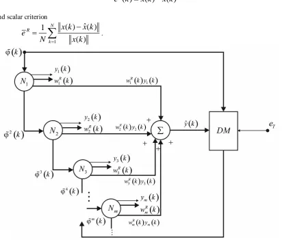
II. ARCHITECTURE OF KERNEL EVOLVING NEURAL NETWORK FOR THE SEQUENTIAL PRINCIPAL COMPONENT ANALYSIS (KENN-SPCA).

The architecture of proposed kernel evolving neural network, the first hidden layer which completely coincides with the first layer of RBFN is shown in fig. 1. Vectors of observations ( )x k 



x k₁( ),…, ( )x k_i ,…,



( )T n

n

x k R , 1 x ki( )1, k1, 2,...,N,... are sequentially fed to radial-basis functions layer 1, formed by bell-shaped kernel activation functions ₁, ₂,…, _l,…, _h,



n+1 h N



, by means of which dimension of the original inputs space is increased.

Fig.1. The architecture of kernel evolving neural network

As such functions traditional Gaussians can be used

2 2

2

l l

x c

l

e





 



and as their centers, in the simplest case sufficiently h randomly are selected cl x l( ) , i.e. vectors-observations can be taken (“lazy” learning [17]). Thus, when the vector of vectors-observations ( )x k is coming at the

input of the system at the output of the first layer vector ( ) k 



1( )k ,…, ( )l k ,…, ( )



T h k

 h

R

 , is formed, where

2

2 (k)

2

( )

l l

x c

l

k

e





 

The second network layer – is layer of centering 2, that realizes elementary transformation

1 1

)

,

( )

( )

k

(k)

(k

(k)

k

k













 











,

(2)

necessary for the effective work of the third layer 3 is formed by an evolving neural network for the on-line principal component analysis and solves the problem of calculating the principal components [19] and eigenvectors. The architecture of the network consists of the Oja’s neurons cascade or their "speed" modifications [16, 17], the decision-making unit DM that, evaluates the number of components m that must be allocated to provide required quality of compression. The output of this layer and KENN-SPCA in general are the current values of the principal components y k₁( ), y k₂( ),…, y_m( )k and eigenvectors of the correlation

matrix ( ) 1 ( )

R R

R k w k , 2

( )

R

w k

,…, R( )

m w k .

Quite a serious problem in the construction KENN-SPCA is effectively forming a basis of radial-basis functions in which informative principal components could be calculate. For this purpose it is necessary to estimate how successful have been selected number h, centers c_l and receptive fields parameters _l of the radial basis functions of the first layer.

This problem of input space recovery layer 4 solves. This layer represents in fact the output layer of radial-basic neural network with h inputs and n outputs and contains nh tuned synaptic weights and n adders.

Thus, the first and fourth layer form RBFN with many outputs that differs from the standard RBFN is the fact that as learning signal here input signal itself is used, i.e. network works as autoassociative system [4]. At the output of the fourth layer signal

x k

ˆ( )



R

n is formed, that is an estimate of the input signal

x k

( )

. The quality of the restoration is estimated by the vector-error using

ˆ

( )

( )

( )

R

e k



x k



x k

and scalar criterion

1

ˆ

( )

( )

1

( )

N

R

k

x k

x k

e

N



x k







.

(3)

If the value R

e exceeds a certain given threshold R T

e , a decision is made that the number of neurons in the first layer should be increased. This process continues until the required recovery quality of the input space had been provide. Results of the fourth layer learning is (n h ) matrix of synaptic weights W N( ), based on the learning dataset containing N observations x k

 

has obtained.

III.KERNEL EVOLVING NEURAL NETWORK FOR SEQUENTIAL PRINCIPAL COMPONENTS ANALYSIS LEARNING

Learning of introduced system can be considered as two relatively independent tasks: radial-basic subsystem self-learning and evolving neural network self-learning for sequential principal components analysis.

The task of the input space recovering consists in finding



n h 



matrix of synaptic weights W

 

wil by

minimizing the learning criterion

2 2

1 1 1

1

1

( )

( )

( )

( )

2

2

k K k

R R R

E

E

x

W

e

  





 



  















(4)

by any of the adaptive algorithms of linear identification, for example, recurrent least squares method

( ( )

(

1) ( ))

( ) (

1)

( )

(

1)

,

1

( ) (

1) ( )

(

1) ( )

( ) (

1)

( )

(

1)

1

( ) (

1) ( )

T

T

T

T

x k

W k

k

k P k

W k

W k

k P k

k

P k

k

k P k

P k

P k

k P k

k









 







_

_{ }









_

_











_

_{ }



_

_



(5)

or any of various modifications.

To improve the quality of input space recovery it is possible, not only adjust the synaptic weights of the fourth layer, but also the parameters of centers cl and widths of the activation functions of the first layer.

Taking into account the obvious relations

 



  

 

 





 

 

  



 

 

 

_{  }

_

 

 

2 2 2 1 2 2 1 1 2 2 2 2 2

(

( )) ,

(

ˆ

1

,

)

(

1

1

(

) ,

2

1

,

2

1

2

)

,

2

l h

i il l

l

h

i i il l

l n R i i l l R i il l l R l l i il l R R l R c

x k

w

k

k

k

x k

w

k

E

k

x k

c

x k

c

E

k

k w

k

x k

c

x k

c

E

k

k

e

k

e

k

e

e

w

k

















   















_



_























_



_









_











 













































it is possible to introduce a recurrent gradient learning algorithms:

 





    



   

 









 





    



   

 





2 2 2 2 1 2 1 2 1 2 2 1 2 2

1

1

1

1

1

1

,

1

l l l

x k c k

k l

l l c i il

l

x k c k

l k

R

R

x k

c k

k

c k

k

k w

k

e

k

x k

c k

k

k

k e

k w

k

e

c

e



where



_c

   

k

,



_

k

- scalar learning rates.

Thus, the relations (5) , (6) form the learning algorithm of all parameters of radial basis neural network with Gaussian activation functions , thus the learning process continues until the desired value of the criterion (3) is riched .

For learning of the second layer expression (2) can be rewritten in the recurrent form:

 

k = (k) - (k);

(k)= (k - 1)+ (

1

( )

k

(k - 1))

k

















.

As is noted above, at the base of third layer are the Oja’s neurons – the adaptive linear associators

N

_j

 

RT

(

1) ( )

y k



w

k





k

and in their learning process. Learning criterion ( energy function ) of the form

 

1

2

ˆ

( )

( )

2

E k





k





k

(7)

is minimized, where

w k

R

( )

- the current estimate of synaptic weights of a neuron , which is , in fact, its eigen assessment of the vector

w

₁R

, ( )

y k

- is current estimate of the first principal component

ˆ( )

k

w k

R

(

1) ( )

y k







of the input signal



( )

k

.

Taking in consideration that the gradient of a criterion (7) by adjustable weights has the form

ˆ

( )

( ( )

( )) ( )

( ( )

( )) ( )

R

R

w

E k



k -



k y k



k - w y k y k



 

 

Oja’s rule for the first principal component can be written as

1

( )

1

(

)

( ) ( )( ( )

1 1

(

) ( ))

1

R R R

w

w k



w k 1

 



k y k



k



w k 1 y k



, (8)

where



_w

( )

k

- learning rate parameter that determines the speed of the algorithm convergence and is usually selected in the terms of the A. Dvorezky’s conditions. In this way, learning rule (8) is stochastic approximation procedure, that characterized by low speed convergence and does not suitable for operation in non-stationary nature of the processed information.

In [16, 17] modifications of Oja’s rule have been introduced

1

1 1 1 1 1

2 1

( )

(

1)

( ) ( )( ( )

(

1) ( )),

( )

(

1)

( ),

0

1,

R R R

w k

w k

r

k y k

k

w k

y k

r k

r k

y k













 











 

 



(9)

that has high performance and additional smoothing properties that are provided by the variable smoothing parameter (forgetting factor)



_.

Using (9) in [18, 19] modifications of Oja’s neuron with the input vector sequence



( )

k

was pothered. Their outputs are the first principal component is

y k

₁

( )

, the first eigenvector

w k

₁R

( )

, and also signals

1

( ) ( )

R 1

w k y k

and



( )

k



w k y k

₁R

( ) ( )

₁





2

( )

k

that need to form of growing cascade of the third layer. Actually third layer of architecture is similar to the Sanger’s neural networks [8] , wherein in the growing casсade of neurons successively calculated first, second and subsequent principal components and eigenvectors .

The learning algorithm of neural network based on procedure (9) can be written in the form 1

2

1 1

1 1

( )

(

1)

( )

( )(

( )

(

1)

( )),

1, 2,..., ,

( )

(

1)

( ),

0

1,

( )

(

1)

( )

( ),

( )

( ),

( )

( )

( ).

R R j R

j j j j j j

j j j

j j R

j j RT j

j j

w k

w k

r

k y k

k

w k

y k

j

m

r k

r k

y k

k

k

w

k y

k

k

k

y k

w

k

k





















 





 











 

 







 







_



(1 0)

From (10) its clear that the first neuron of casсade calculates the first principal component

y k

₁

( )

. Further,

from



( )

k

own projection onto the first eigenvector

w k

₁R

( )

is subtracted 2

1 1

( )

k

w k y k

R

( ) ( )

( )

k









and calculates

y k

2

( )

, that is the first principal component 2

( )

k



or that is the same as the second eigen component of the original signal



( )

k

. The third principal component is calculated by projecting each input vector



( )

k

to the first two eigenvectors that are subtracted from this projection from



( )

k

and finding

3

( )

k



, which is the third main component. The rest of the eigen components of m- th inclusive are calculated recursively according to the strategy that was described.

So the question raises: how many component m must be calculate, to ensure an acceptable level of compression of the original data? That into the third layer of the system have been introduced adder, that calculates «uncompressied» signal



ˆ( )

k

in the form

1

ˆ( )

( )

( )

m R j j j

k

w k y k









,

(1 1)

and decision making element DM in which measure of necessity connection of additional neuron. The quality of the signal recovery (11) is estimated with the help of criterion of type (3) estimated

1

ˆ

( )

( )

1

( )

N

k

k

k

e

N

k















,

the increasing in the number of neurons in layer stops as soon as the controlled signal

ˆ

( )

( )

1

( )

(

1)

(

1)

( )

k

k

e k

e k

e k

k

k















 

_

_





_

_





becomes smaller than a threshold value

e

_T.

IV.CONCLUSION

network that was introduced is easy to implement for solving problems of dynamic data mining (DDM) and data streams mining (DSM).

REFERENCES

[1] Rutkowski L. Computational Intelligence. Methods and Techniques – Berlin - Heidelberg: –Springer - Verlag, 2008. – 514 p.

[2] Du K. - L., Swamy M. N. S., Neural Networks and Statistical Learning. – London: Springer -Verlag, 2014 – 824 p.

[3] Kruse R., Borgelt C., Klawonn F., Moewes C., Steinbrecher M., Held P. Computational Intelligence. – Berlin: Springer, 2013. – 488p.

[4] Ham F.M., Kostanic I., Principles of Neurocomputing for Science and Engineering.–N.Y. : Mc Graw-Hill, Inc. – 2001.– 642 p.

[5] Haykin, S. Neural Networks. A Comprehensive Foundation. / S. Haykin // Upper Saddle River, N.J.: Prentice Hall, Inc., 1999. – 842 р;

[6] Bifet, A. Adaptive Stream Mining: Pattern Learning and Mining from Evolving Data Streams. / A. Bifet // IOS Press. – 2010. – 224 p.

[7] Bodyanskiy, Ye.V. Evolving hierarchical neural network for principal component analysis tasks and its adaptive learning / Ye.V. Bodyanskiy, A.O. Deineko, Sh.V. Deineko, M.O. Shalamov // System tecnologies. – Dnеpropetrovsk. – 2014. – №6 (95). – P. 18-26.

[8] Bodyanskiy, Ye.V., Pliss I. P., Teslenko N. O. Optimal learning algorithm of Oja’s neuron. // Decision making theory. :Proc. of the Inter. сonf. – Uzhgorod. – 2006.–P.10-11. (in Ukrainian)

[9] Bodyanskiy, Ye.V., Pliss I. P., Teslenko N. O. Modification of Oja’s neuron for non-stationary data

analysis // Automation: problems, ideas and solutions.: Proc. of the Inter. сonf. – Sebastopol.– 2006.–

P.17-21. (in Russian)

[10] Bodyanskiy, Ye.V., Pliss I. P., Teslenko N. O. Speed adaptive algorithm for learning of neural that computes minimal component // Information technology and information security in science, technology and education «Infotech-2007»: Proc. of the Inter. сonf. – Sebastopol. – 2007. – V. I. – P. 8-11. (in Russian) [11] Bodyanskiy, Ye.V., Pliss I. P., Teslenko N. O. Hierarchical neural network for principal component

analysis and its adaptive learning // Proc. Int. сonf. «Intellectual systems for decisions making and problems of computational intelligence»– Kherson, 2007. – V.3. – P. 27-29. (in Russian)

[12] Boyko, О.О. Adaptive multistep E. Oja’s and D. Hebb’s self-learning for principal component analysis / О.О. Boyko, M.O. Shalamov, Ye.V. Bodyanskiy // Decision making theory. :Proc. of the Inter. сonf. – Uzhgorod – 2014. – С. 34-35. (in Ukrainian)

[13] Schölkopf B., Smola A. Learning with Kernels. – Cambridge, M.A.:MIT Press, 2002.

[14] Xu, R. Clustering / R. Xu, D. C. Wunsch. // IEEE Press Series on Computational Intelligence. – Hoboken, NJ:John Wiley & Sons, Inc. – 2009. – 341 p.

[15] Bodyanskiy, Ye.V. Adaptive learning of architecture and parameters of radial-basis neural networks / Ye.V. Bodyanskiy, A.O. Deineko // System tecnologies. – Dnеpropetrovsk. – 2013. – №4(87). – P. 166-171. (in Russian)

[16] Bodyanskiy, Ye.V. Adaptive learning of synaptic weights, activation of functions and architecture of radial-basis neural networks / Ye.V. Bodyanskiy, A.O. Deineko, Sh.V. Deineko, I.P. Pliss // Decision making theory. :Proc. of the Inter. сonf. – Uzhgorod. – 2014. – С. 36-37. (in Ukrainian)

[17] Bodyanskiy, Ye.V. Adaptive learning of general regression neural network for processing non-stationary multivariate data sequences / Ye.V. Bodyanskiy, A.O. Deineko, I.P. Pliss // Decision making theory. :Proc. of the Inter. сonf. – Uzhgorod. – 2012. – P. 36-37. (in Ukrainian)

[18] Bodyanskiy, Ye.V. Evolving cascade neural network for sequential principal component analysis and its learning / Ye.V. Bodyanskiy, A.O. Deineko, N.O. Teslenko, M.O. Shalamov // System tecnologies. – Dnеpropetrovsk. – №1(72) – V. 2. – 2011 – Р. 140-147. (in Russian)

[19] Bodyanskiy, Ye.V., Deineko A.O., Teslenko N.O., Shalamov M.O. Evolving cascade neural networks for principal component analysis // Decision making theory. :Proc. of the Inter. сonf. – Uzhgorod. – 2010. – P. 25-26. (in Ukrainian)