association rules mining using heavy itemsets DKE2007

(1)

Elsevier, and the attached copy is provided by Elsevier for the author’s benefit and for the benefit of the author’s institution, for non-commercial research and educational use including without limitation use in instruction at your institution, sending it to specific colleagues that you know, and providing a copy to your institution’s

administrator.

All other uses, reproduction and distribution, including without limitation commercial reprints, selling or licensing copies or access,

or posting on open internet sites, your personal or institution’s website or repository, are prohibited. For exceptions, permission may be sought for such use through Elsevier’s permissions site at:

(2)

Author's personal copy

Association rules mining using heavy itemsets

q

Girish K. Palshikar

a,*

, Mandar S. Kale

b

, Manoj M. Apte

b a

Tata Research Development and Design Centre, Pune 411013, India

b_{Engineering and Industrial Services, Tata Consultancy Services Ltd., Pune 411001, India} Received 9 November 2005; received in revised form 17 February 2006; accepted 18 April 2006

Available online 2 June 2006

Abstract

A well-known problem that limits the practical usage of association rule mining algorithms is the extremely large num-ber of rules generated. Such a large numnum-ber of rules makes the algorithms inefficient and makes it difficult for the end users to comprehend the discovered rules. We present the concept of aheavy itemset. An itemsetAis heavy (for given support and confidence values) if all possible association rules made up of items only inAare present. We prove a simple necessary and sufficient condition for an itemset to be heavy. We present a formula for the number of possible rules for a given heavy itemset, and show that a heavy itemset compactly represents an exponential number of association rules. Along with two simple search algorithms, we present an efficient greedy algorithm to generate a collection of disjoint heavy itemsets in a given transaction database. We then present a modified apriori algorithm that starts with a given collection of disjoint heavy itemsets and discovers more heavy itemsets, not necessarily disjoint with the given ones.

Keywords: Association rules; Data mining; Knowledge discovery in databases; Knowledge compression

1. Introduction

Association rule mining, as originally proposed in [1] with its apriori algorithm, has developed into an active research area. Many additional algorithms have been proposed for association rule mining [2,4,7,16]; see also[10]. Also, the concept of association rule has been extended in many different ways, such as general-ized association rules, association rules with item constraints, sequence rules [11] etc. Apart from the earlier analysis of market basket data, these algorithms have been widely used in many other practical applications such as customer profiling, analysis of products and so on. We have used these algorithms in innovative appli-cations such as warranty claims analysis and inventory analysis. Several commercial data mining tools now offer variants of the association rule mining algorithms.

End users of association rule mining tools encounter several well-known problems in practice. First, the algorithms do not always return the results in a reasonable time. Typically, this happens because the

q

Preliminary version of this paper was published as[9].

* _{Corresponding author. Tel.: +91 20 403 1122; fax: +91 20 404 2399.} E-mail address:[email protected](G.K. Palshikar).

(3)

Author's personal copy

algorithms generate an exponential number of candidate frequent itemsets. Although several different strate-gies have been proposed to tackle efficiency issues, they are not always successful. Also, in many cases, the algorithms generate an extremely large number of association rules, often in thousands or even millions. Fur-ther, the association rules are sometimes very large. It is nearly impossible for the end users to comprehend or validate such large number of complex association rules, thereby limiting the usefulness of the data mining results. Several strategies have been proposed to reduce the number of association rules, such as generating only ‘‘interesting’’ rules, generating only ‘‘non-redundant’’ rules, or generating only those rules satisfying cer-tain other criteria such as coverage, leverage, lift or strength. While these are promising strategies, none of them seem to sufficiently ‘‘compress’’ or reduce the generated association rules, for easy comprehension by end users.

In this paper, we propose a concept called a heavy itemset. An itemsetAis heavy (for given support and confidence values) if all possible association rules made up of items only in Aare present. We prove a simple necessary and sufficient condition for an itemset to be heavy. We present a formula for the number of possible rules for a given heavy itemset, and show that a heavy itemset compactly represents an exponential number of association rules. For example, we show later that if we are able to find a heavy itemset of 20 items in the given transaction dataset, it means that there is no need to outputO(320) association rules, thereby leading to a huge (exponential) decrease in the output size. We present two simple search algorithms and an efficient greedy algorithm to generate a collection of disjoint heavy itemsets in a given transaction database. We then present a modifiedapriorialgorithm that uses a given collection of heavy itemsets and detects more heavy itemsets, not necessarily disjoint with the given ones, and of course the remaining association rules.Table 1shows an exam-ple, where the itemset {‘‘97217’’, ‘‘99501-3095’’, ‘‘98055’’} is heavy (see last 12 rules).

The concept of heavy itemsets is useful in several practical applications; e.g., in a database of inventory or warranty claims, a group of parts (which forms an assembly) will often occur together. For example, when one assembly is replaced, all the member parts in that assembly are actually replaced. Either these relationships among the items will be known beforehand, or they will constitute an interesting new knowledge. (a) If we already know that some parts always occur together, then they can be modeled as heavy itemsets. In this case, the association rules among the member items of an assembly (which are already known) will be suppressed. This is particularly useful when the assembly consists of a large number of parts. (b) Discovering unknown heavy itemsets is a potentially interesting and useful new knowledge. The algorithms presented in this paper can be used to discover only the heavy itemsets in a given transaction database.

The paper is organized as follows. Section2discusses some related work. The formal deﬁnition of the con-cept of heavy itemset and its theoretical properties are discussed in Section 3. Two simple search algorithms and an eﬃcient algorithm to generate a collection of disjoint heavy itemsets are presented in Section4. Section

Table 1

Some association rules generated from real data

‘‘15238-2901’’ )‘‘33610’’

‘‘33610’’ )‘‘15238-2901’’

‘‘28241-7787’’ )‘‘33610’’

‘‘33610’’ )‘‘28241-7787’’

‘‘28241-7787’’ )‘‘98055’’

‘‘98055’’ )‘‘28241-7787’’

‘‘97217’’ )‘‘98055’’

‘‘98055’’ )‘‘97217’’

‘‘97217’’ )‘‘99501-3095’’

‘‘99501-3095’’ )‘‘97217’’

‘‘98055’’ )‘‘99501-3095’’

‘‘99501-3095’’ )‘‘98055’’

‘‘97217’’ )‘‘98055’’, ‘‘99501-3095’’

‘‘98055’’ )‘‘97217’’, ‘‘ 99501-3095’’

‘‘99501-3095’’ )‘‘97217’’, ‘‘ 98055’’

(4)

Author's personal copy

5contains the modiﬁedapriorialgorithm, which uses a given collection of disjoint heavy itemsets as input, and generates ‘‘remaining’’ association rules and also ﬁnds more heavy itemsets, not necessarily disjoint from the given ones. Section 6 presents some experiments results. Section7 presents conclusions and further work.

2. Related work

Association rule mining, as originally proposed in [1] with its apriori algorithm, has developed into an active research area. Many additional algorithms have been proposed for association rule mining [2,4,7,16]; see also [10]. End users of association rule mining tools encounter several problems in practice, such as too much time taken by the algorithms and too many rules generated as output. Since finding support requires a pass over the entire database (and thus results in high I/O cost), one strategy to improve the efficiency involves the use of random sampling to estimate the support of an itemset; see[6,14]. Use of hash-based effi-cient data structures [13] and mining of vertical (rather than horizontal) database [12] are some other approaches that have been tried to improve the efficiency of the association rule mining algorithms.

Ref.[17]compared five well-known association rule mining algorithms (viz.,apriori, FP-tree, charm, Mag-num-Opus and Closet) using three real-world data sets and observed super-exponential growth in the number of rules generated on these datasets. Several different strategies have been proposed to reduce the number of association rules generated. For example, we could use an interestingness measure to generate only interesting rules. See[5]for a survey of many interestingness measures proposed in the literature. A closely related work is [15], which proposed the concept of a closed frequent itemset and used it to generate an exponentially smaller number of non-redundant association rules. Several post-processing strategies have been proposed in [8] to reduce the number of generated association rules; e.g., prefer general association rules over specific ones, sum-marize and report onlydirection-setting(i.e., rules which indicate the type of correlation between specific item-sets) rules etc. In[3], algorithms are given to find itemsets containing highly correlated items i.e., association rules having high confidence but not constrained by any minimum support.

In this paper, we are nottrying to reduce the number of association rules by choosing some of them and ignoring the others. Instead, we focus on the problem of compactly representing the association rules by means of heavy itemsets. Broadly, our approach is summarized as original association rules = heavy item-sets + remaining association rules. Note that all original association rules can be recovered, if desired, from the outputs of our algorithms.

3. Heavy itemset

When generating association rules over a set of items, we often ﬁnd that all possible association rules over a subsetAof items are generated. Each of these association rules overAhas the formX)YwhereXandYare disjoint non-empty subsets ofA. These rules clutter the generated output. They can be actually summarized (and hence removed from the output) by stating that Ais a heavy itemset.

Deﬁnition 1. LetLandRbe any two non-empty disjoint itemsets. Let 0.0 <r,s6_{100.0 be the given support}

and conﬁdence values. We say thatL)Ris a valid association rule(for givenrand s) if (i) support(L)Pr

and (ii) support(L[R)Prand (iii) [support(L[R)/support(L)]Ps.

Deﬁnition 2. Let 0.0 <r, s6_{100.0 be the given support and conﬁdence values. A non-empty itemset} _A

(jAjP2) is said to be a heavy itemset (for given r and s) if for every non-empty disjoint subsets X, Y of A,X)Yis a valid association rule (for givenrands). An element of a heavy itemset is called a heavy item. It is easy to see that a subset (of cardinality 2 or more) of a heavy itemset is itself a heavy itemset. This observation, along with the efficient condition for checking whether a given itemset is heavy or not (as proved below) leads to a straightforward application of theapriorialgorithm for mining only heavy itemsets. In each step of apriori, instead of finding frequent itemsets, we find heavy itemsets. However, we run into the same

(5)

Author's personal copy

We ﬁrst formalize the concept of heavy itemset, so as to facilitate counting of the rules a heavy itemset represents.

Deﬁnition 3. Given a non-empty ﬁnite setA= {a1,a2,. . .,an} ofnP2 items. A 2-split(or simply, asplit) ofA

is a tuple (X,Y) whereX,Yare non-empty disjoint subsets of A(i.e.,X,YA,X5;,Y5;andX\Y=; butX[Yneed not be all ofA).A split-setoverAis a non-empty set of splits ofA. Given a non-empty subset BA, the complete split-set of Bis the set of all splits of B.

For example, let A= {a,b,c,d}. Then ({a}, {b,d}) is a split of A and so are ({b}, {d}), ({d}, {b}) and ({b,c}, {a,d}). The complete split-set of B= {a,b,c} containing 12 splits is

fðfag;fbgÞ;ðfag;fcgÞ;ðfbg;fagÞ;ðfbg;fcgÞ;ðfcg;fagÞ;ðfcg;fbgÞ;ðfag;fb;cgÞ;ðfbg;fa;cgÞ;ðfcg;fb;agÞ; ðfa;bg;fcgÞ;ðfa;cg;fbgÞ;ðfb;cg;fagÞg

Thus a split represents an association rule; e.g., the split ({a}, {b,c}) stands for the association rule {a}){b,c}. Then an itemsetAis heavy if all the association rules in the complete split-set ofAare present with the required support and conﬁdence.

Proposition 1. The size of the complete split set (i.e., the number of all possible splits) for a given finite set A of size N is given by

XN

m¼1 X

Nm

n¼1

N_C

mNmCn: ð1Þ

Here, m and n denote the sizes of the LHS and RHS sets in a spilt.

Proof. The term NCmdenotes the number of ways in which the m elements in the left hand side set can be

selected out of the total N elements. The term NmCn denotes the number of ways in which the n elements

in the right hand side set can be selected out of the remainingNmelements. Since both LHS and RHS need to be selected, we take the product of these two terms (rule of product). Since the number of elementmvaries from 1 toNandmvaries from 1 toNm, we take the summations over all possible values ofmandn, to get the total number of splits sets (rule of sum). When m=N, we assume that the term 0Cn= 0. h

Thus, if N= 3 (e.g., A= {a,b,c}), the total number of all possible splits is 3C1Æ(2C2+ 2C1) + 3C2Æ (1C1) = 3Æ3 + 3Æ1 = 12, as shown above. IfN= 4, the total number of possible splits is

4_C

1 ð3C3þ3C2þ3C1Þ þ4C2 ð2C2þ2C1Þ þ4C31C1 ¼4 ð1þ3þ3Þ þ6 ð1þ2Þ þ41 ¼28þ18þ4¼50:

It is easy to provide an upper bound on the summation inProposition 1. Each item in the itemsetAhas three choices for each split: either it appears in the left side or it appears in the right side or it does not appear in either side. Thus the total number of possible rules for an itemset Aof sizen is bounded above by 3n. Since neither the RHS nor the LHS of an association rule can be empty, we need to eliminate such association rules. The number of association rules where the RHS is empty and the LHS is any subset of the itemset is 2n. Sim-ilarly, the number of association rules where LHS is empty is also 2n. Since the empty association rule (LHS = RHS =;) is counted twice, an alternative expression for the number of association rules correspond-ing to a heavy itemset of n items: 3n2n+1+ 1. This expression is equivalent to the one inProposition 1. Corollary 2. A heavy itemset compactly represents an exponential number of association rules.

Proof. Immediately follows from the expression 3n2n+1+ 1 for the number of association rules correspond-ing to a heavy itemset of n items proved in the preceding paragraph. h

The signiﬁcance of a heavy itemset is then as follows. If we identify an itemsetHas heavy, then we need not report the association rules corresponding toH. Thus identifying a heavy itemset enables an exponential com-pression in the number of association rules reported by an algorithm for mining association rules.

(6)

Author's personal copy

Proposition 3. Suppose H ={a1, a2,. . ., an} is an itemset of nP2 items. Let s0 be the support of H. Let s1, s2,. . ., sn be the supports of the singleton itemsets {a1},{a2},. . .,{an}, respectively. Let the minimum required support and confidence berands. Let mn =min{s0, s1, s2,. . ., sn}and mx =max{s0, s1, s2,. . ., sn}be the minimum and maximum of the support values. Then H is a heavy itemset iff (i) mnPr and(ii)(mn/mx)Ps.

Proof. (only-if part) Assume that (i) mnPr and (ii) (mn/mx)Ps. H is a heavy itemset iffL)Ris a valid association rule for any disjoint non-empty subsetsLandRofH. LetLandRbe any two disjoint non-empty subsets ofH. We need to prove that (i) support(L)Prand (ii) support(L[R)Prand (iii) [support(L[R)/ support(L)]Ps. Clearly, support(L)Pmn. Given thatmnPr, it follows that support(L)Pr. Similarly, we can prove that support(L[R)Pr. [support(L[R)/support(L)]Pmn/support(L)Pmn/mx which is given to bePs; hence [support(L[R)/support(L)]Psas required. HenceL)Ris a valid association rule. Since L, Rare arbitrary disjoint subsets of H, we have proved thatH is a heavy itemset.

(if part) Assume thatH is a heavy itemset. We need to prove that (A)mnPrand (B) (mn/mx)Ps. Since mx= max{s0,s1,s2,. . .,sn}, letL= {ak} be the singleton itemset such that support(L) = support({ak}) =mx.

LetR=HnLbe the itemset of all items fromHexceptak. Clearly,L,Rare two disjoint subsets ofHsuch that L[R=H and L\R=;. Then since H is a heavy itemset, L)R is a valid association rule. Hence, (i) support(L)Pr and (ii) support(L[R)Pr and (iii) [support(L[R)/support(L)]Ps. Since sup-port(L[R) =s0=mn, it follows from (ii) thatmnPr, thus proving (A) we now prove that (B) mn/mxPs. In (iii), the numerator is the same as mn and the denominator is the same as mx and hence it follows by substitution thatmn/mxPs. h

We present below an algorithm that returns yes or no depending on whether or not the given itemset is heavy. Note that the algorithm uses the condition proved in Proposition 3 and does notexplicitly check all the possible association rules to decide whetherH is heavy or not.

algorithm is_heavy // checks whether given itemset is heavy or not input databaseDof Ntransactions

input itemset H= {a1,a2,. . .,an} ofnP3 items

input minimum support r, minimum conﬁdences

output yes ifH is a heavy itemset;no otherwise 1. Lets0be the support of H in D;

2. Lets1,s2,. . .,sn be the supports of {a1}, {a2},. . ., {an} inDrespectively;

3. Letmn= min{s0,s1,s2,. . .,sn} andmx= max{s0,s1,s2,. . .,sn} be the minimum and maximum of the support

values;

4.if mn<rthen return(no); 5.if (mn/mx<s) thenreturn(no); 6.return(yes);

Correctness of the algorithm follows from Proposition 3. Checking this condition for a given itemset

A requires one pass over the database to obtain support for each of the singleton subset of A (which needs to be done once only) and for A itself. The algorithm’s complexity is O(N), where N= no. of transactions.

4. Finding disjoint heavy itemsets

In this section, we present three different approaches to find out a disjoint collection of heavy itemsets. The first two approaches are more conceptual and the third is more suited for practical applications, since it is based on a well-known efficient data structure called FP-tree.

4.1. Searching the subset tree

(7)

Author's personal copy

Deﬁnition 4. LetF1be the set ofjF1j=nfrequent itemsets in a given transaction database (for a given support and conﬁdence). A collection of pairwise disjoint subsets of F1 is called a sub-partition ofF1. A heavy-sub-partition ofF1is a sub-partitionPofF1, where each element ofPis a heavy itemset. A heavy-sub-partitionC of F1 is maximal if no subset of F1 [Cis heavy, where [Cdenotes the union of all elements ofC.

Without loss of generality, assume that the items in F1 are numbered 1, 2,. . .,n. As an example,

C= {{1, 2, 5}, {4, 8}} is a sub-partition of the set F1= {1, 2, 3, 4, 5, 6, 7, 8, 9}; here, [C= {1, 2, 5, 4, 8}. Given

F1, we need an algorithm to ﬁnd a maximal heavy-sub-partition of F1. We later give examples to illustrate the fact that there is no unique maximal heavy-sub-partition for a given F1i.e., a given F1 may have many diﬀerent maximal heavy-sub-partitions.

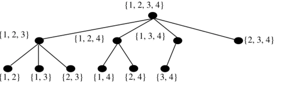
All possible subsets ofF1 can be arranged in a standardsubset tree. A vertexu in the subset tree ofF1 is labeled with a subset AF1; this vertex u has at mostjAj children, each of which is labeled with a subset of A having size jAj 1. These children of u are arranged from left to right, as per the numeric order of the subsets, assuming that elements within each subset are sorted in ascending order. If any of thesejAjsubsets has already occurred in the subtree of the left siblings ofuthen it is not added as a child foru. The root of the subset tree is labeled with the entire set F1. We stop expanding the tree whenjAj= 2.

Fig. 1shows the subset tree for F1= {1, 2, 3, 4}. The following properties of a subset tree are obvious.

Proposition 4. Each subset of F1of sizeP2 appears exactly once in the subset tree of F1. Also, the number of vertices in the subset tree of a set of size n is 2nn1 = O(2n).

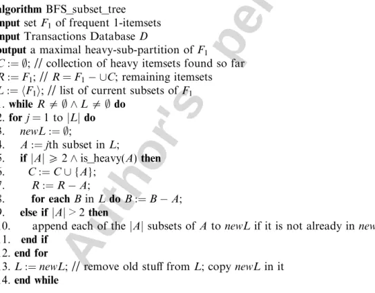
We can devise a simple algorithm to ﬁnd a maximal heavy-sub-partition of a given set F1. This algorithm essentially performs an implicit breadth-ﬁrst search of the subset tree ofF1; the search is implicit in the sense that the entire subset tree is not constructed apriori before the search. In each iteration, this algorithm con-structs all children of a particular node and tests each of them for heavy itemset. If a heavy itemset is found, it is added to the collection of heavy itemsets found so far, removes the items in it from the set of items avail-able for further construction of subsets. The algorithm stops when there are no more subsets to check. algorithm BFS_subset_tree

input set F1of frequent 1-itemsets

input Transactions Database D

output a maximal heavy-sub-partition ofF1

C:¼ ;; // collection of heavy itemsets found so far

R:¼F1; // R=F1 [C; remaining itemsets

L:¼ hF1i; // list of current subsets of F1 1.while R5; ^L5; do

2.for j= 1 to jLj do 3. newL:¼ ;;

4. A:¼jth subset in L;

5. ifjAjP2^is_heavy(A) then 6. C:¼C[{A};

7. R:¼RA;

8. for each Bin Ldo B:¼BA; 9. else if jAj> 2 then

10. append each of thejAj subsets ofAto newL if it is not already in newL; 11. end if

12. end for

13. L:¼newL; // remove old stuﬀ fromL; copy newL in it 14. end while

In the worst case, the above algorithm has to visit all vertices of the subset tree, which areO(2n), where

(8)

Author's personal copy

It is easy to see the above algorithm has no ‘‘focus’’ while searching the subset tree. For example, if {3, 4} were a heavy itemset then the algorithm would reach it only after searching the previous (left) sub-trees, such as the sub-trees rooted at {1, 2, 3} and {1, 2, 4}. It is possible to use diﬀerent strategies, such as depth-ﬁrst, to search the subset tree.

4.2. Searching the heavy itemset tree

We now present another algorithm that performs a depth-ﬁrst search of the subset tree in a bottom up man-ner. Notice that each node in the subset tree is really a candidate heavy itemset. The next algorithm uses a pruning strategy to reduce the search space. Given a candidate heavy itemsetH, the idea is to consider only those of the remaining items that can possibly be added toH.

{1, 2, 3} _{{1, 2, 4}} _{{1, 3, 4}}

{2, 3, 4}

{1, 2} {1, 3} {2, 3} {1, 4} {2, 4} {3, 4} {1, 2, 3, 4}

Fig. 1. The subset tree forF1= {1, 2, 3, 4}.

algorithm heavy1 // try to ﬁnd a heavy itemset of given sizek

input D// transaction database input r, s // support and conﬁdence input F1 // set of frequent items

input k// desired number of items inH

input L // items which can be added next toH

input CH // the heavy itemset (of size <k) constructed so far

1.L1:¼set of all itemsJinLbut not in CH such that support of CH[{J}Prarranged in descending order of support

2.if (jL1[CHj<k) then return ;endif 3.for every item I2L1 do

4. if(get_conﬁdence(CH[{I})Ps) then 5. if(jCH[{I}j==k) then

6. return CH[{I}

7. else

8. H:¼heavy1(D,r,s,F1,k,L1n{I}, CH[{I}) // recursive call 9. if (H! =;) then return Hendif

10. endif

11. endif 12.endfor 13.return ;

algorithm ﬁnd_disjoint_heavy_itemsets_simpliﬁed input D// transaction database

input r, s // support and conﬁdence

outputS // collection of disjoint heavy itemsets

1. LetF1:¼the list of frequent 1-itemsets inDarranged in descending order of support 2.S:¼ ;

(9)

Author's personal copy

We recursively deﬁne a vertex-labeled, rooted tree called theheavy itemset tree Tas follows.

Deﬁnition 5. Each node in heavy itemset tree T is labeled with a candidate heavy itemset CH and an itemset L1 disjoint from CH, indicating the items that can be added to CH. The root of T is labeled with CH =; and L1 =F1, whereF1 is the set of all frequent items in the given transaction database. Each node has a child for every item in L1. The candidate heavy itemset for a child is CHa= CH[{a}, for an item a2L1.

It is easy to see that the algorithm heavy1 implicitly constructs and performs a depth-ﬁrst search of the heavy itemset treeT. At a particular level of recursion, the algorithmheavy1 constructs and searches all chil-dren ofTat that level. The depth of this tree is at mostk, because the size of CH is incremented by 1 at each level and the algorithmheavy1 stops when it reaches a vertex inTwithjCHj=kand when that CH is indeed a heavy itemset. For a vertexuinTat depthm, the algorithm does not create and search any of its child vertices, if size of the listL1 atuis not enough to reach the ‘‘remaining’’ depthkmi.e., no leaf in the sub-tree atucan have CH of size k(mis also equal to the size of CH at that level).

Lemma 5. Every subset of size k of the set F1 at the root of the tree T either(i) occurs as a candidate heavy itemsetCHfor some leaf in T or(ii)it is certain that it is not heavy. Formally, we need to prove that every subset of size m of the set F1 is either the CH for some vertex of T at level m + 1 or it is not heavy.

Proof. See Appendix A. h

Proposition 6. Algorithm heavy1 terminates, returning a heavy itemset H where HF1 andjHj= k and return-ing ;if no such heavy itemset exists.

We can improve the performance ofheavy1 by adopting the strategy used inapriori. Assume that each item has a unique integer ID. Then we can replace Line 1 in heavy1 by the following line, which would reduce repeated construction of already tested itemsets.

1. L1:¼set of all itemsJin Lbut not in CH such that support of CH[{J}PrandJ> every ID in CH in ascending order of item IDs.

Proposition 7. Algorithm find_disjoint_heavy_itemsets_simplified terminates, returning a collection S containing disjoint heavy itemsets. Moreover, the algorithm finds and reports one of the largest itemsets i.e., if the algorithm reports the largest heavy itemset of size say k, then there is no heavy itemsets of size k + 1.

We remark that the above algorithm ﬁnds and returns the heavy itemset having the maximum size; how-ever, we do not say anything about the size of the other heavy itemsets returned.

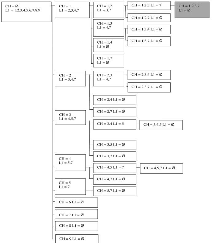
The worst case for the above algorithm will be such that almost the entire heavy itemset tree is traversed. One way in which this can happen is as follows. Consider the situation where the setF1 containsMfrequent items and everym-size subset (except one) ofF1 is heavy and no subset ofF1 of size (m+ 1) is heavy. In this case, almost the entire heavy itemset tree up to depthmwill be traversed and this means that an exponential number of nodes are examined by the algorithm heavy1 (when called with k=m+ 1).

Fig. 2shows the heavy itemset tree searched by this algorithm on the transaction database in Table 2. 4. whilejF1j>k do

5. H:¼heavy1(D,r,s,F1,k,F1,;) // try to ﬁnd a heavy itemset of sizek

6. if(H! =;) thenS:¼S[{H};F1:¼F1nH else break endif // addH to S

(10)

Author's personal copy

4.3. FP-Tree

We can use any association rule mining algorithm to detect all heavy itemsets from the data. We only need to add a check for heavy itemset, once a frequent itemset is found. Diﬀerent association rule mining algorithms have diﬀerent strengths and weaknesses in practice, though all seem to have the same worst-case behaviour. Frequent pattern (FP) tree algorithm [4]seems more suitable for adaptation for fast detection of large heavy itemsets, because of the following reasons: (a) it is not a level-wise algorithm unlikeaprioriand others; (b) it

CH = Ø

L1 = 1,2,3,4,5,6,7,8,9

CH = 1 L1 = 2,3,4,7

CH = 1,2 L1 = 3,7

CH = 1,2,3 L1 = 7

CH = 1,2,7 L1 = Ø CH = 1,3

L1 = 4,7 _{CH = 1,3,4 L1 =}_Ø

CH = 1,3,7 L1 = Ø CH = 1,4

L1 = Ø

CH = 1,7 L1 = Ø

CH = 2 L1 = 3,4,7

CH = 2,3 L1 = 4,7

CH = 2,4 L1 = Ø

CH = 2,7 L1 = Ø

CH = 2,3,4 L1 = Ø

CH = 2,3,7 L1 = Ø

CH = 3 L1 = 4,5,7

CH = 3,4 L1 = 5

CH = 3,5 L1 = Ø

CH = 3,7 L1 = Ø

CH = 3,4,5 L1 = Ø

CH = 4 L1 = 5,7

CH = 4,5 L1 = 7

CH = 4,7 L1 = Ø

CH = 4,5,7 L1 = Ø

CH = 1,2,3,7 L1 = Ø

CH = 5 L1 = 7

CH = 5,7 L1 = Ø

CH = 6 L1 = Ø

CH = 7 L1 = Ø

CH = 8 L1 = Ø

CH = 9 L1 = Ø

(11)

Author's personal copy

works well on itemset space as well as transaction space and (c) seems suitable for storing and analyzing dense data.

We present a modiﬁed FP-tree algorithm to detect a disjoint collection of heavy itemsets in given transac-tions. Intuitively, the modiﬁcations are as follows:

• We force it to look for heavy itemsets of speciﬁc size, instead of discovering all heavy itemsets; and • Once a heavy itemsethis found, we ignore all items fromhwhile doing further analysis, thereby leading to

a discovery of disjoint heavy itemsets.

Thus we modify the FP-tree algorithm to detect a collection H of large disjoint heavy itemsets from the given transactions. Once such a collectionHis available, we show later how to modify of theapriorialgorithm to discover all remaining association rules, along with any remaining heavy itemsets, not necessarily disjoint from those in H.

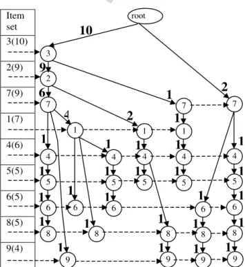
We ﬁrst summarize the concept of the frequent-pattern tree, introduced in[4]. Afrequent-pattern tree( FP-tree) consists of (i) aheader, which is a sorted list of frequent itemsets in the descending order of their support, (ii) vertices consisting of items in the header, (iii) solid edge from an itemu to itemvhaving a link count c if support ofuPsupport ofvandu andvco-occur inctransactions, (iv) dashed edge from each itemu in the header to the ﬁrst vertex in the tree foru, (v) dashed edge from each vertexuto the next vertex foruin the tree. Thus, all the vertices in the tree for the same item u are ordered from left to right and connected into a sequence by dashed edges. Dashed edges do not have any count values. An FP-tree is a representation of all the transactions pruned to contain only items in its header. Support for an item u in the header is equal to the sum of the link counts of all solid edges that come into a vertex in the tree labeled withu. The algorithm for constructing an FP-tree is as follows. For simplicity, we omit the construction of the header of FP-tree, which contains frequent items in the given transaction database and their links.

algorithm build_fp_tree

input Transactions Database D

output FP-TreeT

1. Create a root node Tof FP-Tree and label it asnull

2.for every transaction t2Ddo 3. ift is not empty then 4. insert (t,T)

5. link new nodes to other nodes with similar labels links originating from header list 6. endif

7.end for

8.return FP-TreeT

Table 2

Transaction, frequent 1-itemsets and pruned transactions

Original transactions Frequent 1-itemsets item (support) Pruned, sorted transactions

2, 3, 4, 5, 6, 7, 8 3 (10) 3, 2, 7, 4, 5, 6, 8

4, 5, 6, 7, 8, 9 2 (9) 7, 4, 5, 6, 8, 9

1, 2, 3, 4, 5 7 (9) 3, 2, 1, 4, 5

1, 2, 3, 6, 7 1 (7) 3, 2, 7, 1, 6

1, 2, 3, 7 4 (6) 3, 2, 7, 1

1, 2, 3, 7, 8 5 (5) 3, 2, 7, 1, 8

2, 3, 7, 9, 10, 11 6 (5) 3, 2, 7, 9

1, 2, 3, 4, 5, 6, 7 8 (5) 3, 2, 7, 1, 4, 5, 6

6, 7, 8, 9, 10, 11 9 (4) 7, 6, 8, 9

1, 2, 3, 4, 8, 9, 10, 1 3, 2, 1, 4, 8, 9

1 3, 2

2, 3 3, 7, 1, 4, 5

(12)

Author's personal copy

First column of Table 2 shows a database containing N= 12 transactions of 11 items. For r= 33%,

s= 33%, the 9 frequent 1-itemsets are shown in column 2 of Table 2. Column 3 of Table 2 shows each of the original transactions after (i) pruning the infrequent items (10, 11) and (ii) sorting the remaining items in the transaction in descending order of their support. Fig. 3shows the FP-tree for these pruned and sorted transactions.

Thepath labelfor a path in an FP-tree is the minimum link count in that path; e.g., inFig. 3, the path label of the path hroot, 3, 2, 7, 1i is min{10, 9, 6, 4} = 4.

Given an itemuin the header of an FP-treeT, we construct a new conditional FP-treeTuforuas follows. Tuis the same asTexcept that it does not contain any vertex labeled withv(and solid edges incident on them) wherevcomes ‘‘after’’uin the header ofTor there is no path inTfrom the root to the vertexvwhich passes through u. The later condition essentially removes those transactions in whichu is not present. Such itemsv

are also removed from the header ofTu. The link counts inTuand support values for items in the header are diﬀerent from those inT; these are initialized to 0 and re-calculated as follows. Consider the frequent item 1; there are three pathsh3, 2, 7, 1i,h3, 2, 1i,h3, 7, 1ito the three vertices labeled 1 in the FP-treeTofFig. 3. These paths represent a total of seven transactions, since support(1) = 7 in the header of T. The path label for h3, 2, 7, 1iis 4; so add 4 to each link count in this path. The path label for h3, 2, 1i is 2; so add 2 to each link count in this path. Finally, the path label forh3, 7, 1iis 1; so add 1 to each link count in this path. Now we ﬁnd algorithm insert

input transactiont, any_node 1.while t is not empty do

2. ifany_node has a child node with labelhead(t) then

3. increment link count between any_node and head(t) by 1 4. else

5. create a new child nodeT0 of any_node with labelhead(t) and having link count 1 6. endif

7.end while

8.call insert(body(t),T0)

root 3 Item set 3(10) 2(9) 7(9) 1(7) 4(6) 5(5) 6(5) 8(5) 9(4) 2 7 9 4 5 6 8 1 6 8 4 5 6 1 4 5 8 9 7 1 4 5 6 8 9 7 4 5 6 8 9

9

6

1

4

1

10

1

2

1

2

1 ₁

1

(13)

Author's personal copy

the new support for an item u in the header ofTuas the sum of the link counts of all solid edges that come

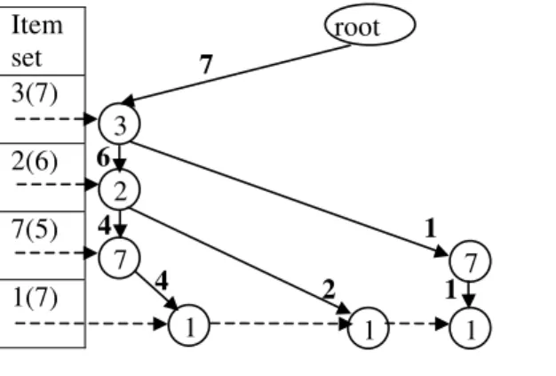
into a vertex in the conditional FP-tree labeled with u. Fig. 4 shows the conditional FP-tree for frequent item 1.

4.4. Finding disjoint heavy itemsets using FP-Tree

We now present an FP-tree based algorithm to ﬁnd a collection ofdisjointheavy itemsets for a given data-base D, support rand conﬁdences.

algorithm ﬁnd_disjoint_heavy_itemsets input databaseDof Ntransactions. input support s, conﬁdence t

output a collectionSof disjoint heavy itemsets

1.S=;; h=;; // h= current heavy itemset being built 2. (HD,T) = build_fp_tree(D) //HD is the header

3.nDepth=jHDj; // size of heavy itemset we are looking for 4.nHeavy=jHDj; // size of largest possible heavy itemset 5.while (nDepth> 1) do

6. if(jhj> 0)then// found heavy itemset h

7. S=S[{h};h=;; // add hto S, re-initialize hto empty 8. delete all elements ofh from HD

9. re-initialize all links in HD to NULL 10. nHeavy=nHeavy jhj

11. nDepth=nHeavy

12. Delete the old FP-treeT

13. T= build_fp_tree(HD, D) // build new FP-tree 14. endif

15. forevery item I in HDdo // start from last item 16. conditional_treeR (T,HD, I, r, s, nDepth, ;, h)

17. nHeavy=nHeavy–1

18. if nHeavy<nDepth then break; endif 19. end for

20. nDepth=nDepth–1 21. end while

22. returnS

algorithm conditional_treeR

input T, HD, I, r, s, nDepth // FP_tree, header, item, support,. . . root

3 Item set 3(7)

2(6)

7(5)

1(7) 2

7

1 1

7

1 6

4

4 7

2

1

(14)

Author's personal copy

The subroutine build_fp_tree is the same as the one in[10]. The subroutine get_conﬁdence computes the conﬁdence of an itemset A_{as per the formula 100 * (support(}A)/mx), wheremx= max{support of elements of A}.

We now illustrate our algorithm for finding heavy itemsets. Initially, nDepth=nHeavy= 9, which is the number of frequent 1-itemsets. The subroutine conditional_treeR builds the conditional FP-tree T1 for item 9 and finds that there are no other items in the header HD1 of T1. The condition in line 6 is violated, the subroutine returns, nHeavy is decremented, condition in line 17 is violated, the for loop is exited. Thus there is no possibility of getting a heavy itemset of size 9. Hence nDepth is decremented and the algorithm starts looking for a heavy itemset of size 8. The algorithm continues and does not find any heavy itemsets of size upto 5 or more. Suppose nDepth=nHeavy= 4. The algorithm does not find any heavy itemset of size 4 for conditional FP-trees of items 9, 8, 6, 5, 4. Suppose now I= 1 in line 14 in find_disjoint_heavy_itemsets. We now enter the subroutine conditional_treeR and build the conditional FP-tree for 1 (Fig. 4).

No item is removed from HD1 in line 2. Now L= {1} and CH = {3, 2, 7, 1}. Since support({1}) = 4, the get_conﬁdence condition is satisﬁed in line 9. We now recursively enter subroutine conditional_tree, with

I1 = 7. In the recursive call, conditional FP-tree for 7 is built using the conditional FP-tree for 1, whose header containsHD1 = {3, 2, 7}, none of which are removed in line 2. NowL= {1, 7}, CH = {3, 2, 7, 1}. Since sup-port({1, 7}) = 4 (as per the conditional FP-tree of 7) and max{support({1}), support({7}) = 9, as per the header in original FP-treeT_{, conﬁdence = (4/9) * 100 = 44.44 > 33%. Continuing similarly, we reach and}

sat-isfy the base condition for recursion in line 23; thus finding and reporting the heavy itemset {3, 2, 7, 1}. These four items are then removed from the header of the original FP-tree and the algorithm continues, finding another heavy itemset {4, 5}. The algorithm stops after reachingnDepth= 1 in find_disjoint_heavy_itemsets. The worst-case complexity of the algorithm find_disjoint_heavy_itemsets is the same as that of the original FP-tree algorithm (exponential in the worst case).

input L // list of items for which conditional tree is built

outputh; // heavy itemset found (his both an input and output parameter) 1. (HD1,T1) = build_conditional_fp_tree(T,HD,I)

2. Remove all elements of HD1 for which the support of the item (as perT1) in the element is <r. 3.L=L[{I}

4. CH =L[HD1 // candidate heavy itemset 5.nHeavy=jCHj

6.if (nHeavy<nDepth)then return 1 endif// don’t record this itemset on return path 7.if (jHD1j> 1)then

8. if(get_conﬁdence(L) <s)then return 0 endif 9. found= 0;

10. forevery item I12HD1 such that I15Ido

11. rec= conditional_treeR(T1,HD1,I1,r,s,nDepth,L,h) 12. if (rec! = 0)thenfound= 1endif;

13. nHeavy=nHeavy1

14. if (nHeavy<nDepth) then return 1 endif 15. end for

16. if(found== 0)then

17. if (get_conﬁdence(L) >s) then{h=h[L; return1;} 18. else return 0;endif

19. else return1; endif // found something during recursion, so return 1 22.else // come here whenjHD1j6₁

23. if (get_conﬁdence(L) >s) then{h=h[CH;rec= 1;} 24. else rec= 0;endif

(15)

Author's personal copy

5. The apriori_heavy algorithm

We have observed in practice that, in general, a given transaction database contains non-overlapping (i.e., non-disjoint) heavy itemsets; e.g., {3, 9} and {2, 5, 7, 9}. Thus the goal is to detectallheavy itemsets in the given transactions, not only the disjoint heavy itemsets. We presented earlier a modiﬁed FP-tree algorithm to detect a collection Hof large disjoint heavy itemsets from the given transactions. Once such a collection His avail-able, we now show a modiﬁcation of the apriori algorithm to discover all remaining association rules, along with allremaining heavy itemsets, not necessarily disjoint from those in H.

SupposeAis the set of all frequent 1-itemsets in a given transaction databaseD. Suppose also that we ﬁnd a collection H= {h1,h2,. . .,hk} ofkheavy itemsets in Dusing the above algorithm. LetBbe the set of all

fre-quent items inA, which do not occur in any heavy itemset inS. Apart from the association rules consisting of items only inB, there may be additional association rules involving (i) relationships between items in different heavy itemsets in H; and (ii) relationships between items inBand items in one or more heavy itemsets in H. We now give an association rule mining algorithm, which usesHandBas given inputs and finds the set of all other ‘‘missing’’ association rules. The algorithm also finds more heavy itemsets, not necessarily disjoint from the given ones and adds them toH. Thus the generated collection of heavy itemsetsHand the generated asso-ciation rules complete the mining process.

algorithm apriori_heavy

input set of heavy itemsets H= {h1,h2,. . .,hk} // known heavy itemsets;H can be;

input set of frequent itemB= {f1,f2,. . .,fm} where each {fi} is a frequent 1-itemset andfi62hj, for anyhjinH

input transaction databaseD, support r, conﬁdences

output set of association rulesL)R

output H// more heavy itemsets are added to H given as input

1.C2= {{u,v}j($16i, j6ksuch that u2hi^v2hj^i5j)_($16i6m, 16j6ksuch that u=fi^v2hj)_($16_i_,_j6_m_{such that} _i₅_j^_u₌_fi^_v₌_fj_)}

2. Find support of all 2-itemsets in C2 to determineL2 3. move_to_heavy(L2,H)

4.k:¼3;stop= 0; 5.while stop= 0 do

6. Ck= gen_candidate_itemsets(H,B,k,Lk1) 7. prune(Ck,H,B)

8. Lk= set of all candidates inCkhaving supportPr

9. ifLk=; thenstop= 1; endif 10. move_to_heavy(Lk,H)

11. end while 12. k++

13. answer =[Lk

algorithm move_to_heavy

input Lk, H // lists of frequent k-itemsets and heavy itemsets 1.for all itemsets l2Lkdo

2. ifis_heavy(l) then 3. H=H[{l}

4. Remove all strict subsets of lfrom H

5. Lk=Lk{l} 6. endif

7.end for

algorithm gen_candidate_itemsets

(16)

Author's personal copy

The algorithmapriori_heavyis nearly the same as the originalapriorialgorithm, except for the following. The initial candidate itemsets are of size 2, obtained by taking pair-wise Cartesian product of the heavy item-sets in Hamong themselves and with the set Bof ‘‘non-heavy’’ frequent items. After ﬁnding the frequentk -itemsets, the algorithm checks (using subroutine is_heavy) if any of them are heavy itemsets; if so, then it removes that set fromLkand adds it toH, taking care to remove all proper subsets of the newly added heavy itemset fromH. Since the setLkmay become empty in this process, the terminating condition stated diﬀerently

(stop when no new frequent itemsets are found).

In algorithm gen_candidate_itemsets, lines 2–7 are the nearly same as the original candidate generation scheme in apriori; except that heavy itemsets of sizek1 are also treated as frequent (k1)-itemsets. Rest of the lines 7–17 pick a frequent (k1)-itemset (or a (k1) size heavy itemset fromH) and systematically add one heavy element from H to it. The itemsets are assumed to be sorted as per the (arbitrary) item IDs. A small modiﬁcation is needed to actually generate the association rules from the resulting heavy itemsets and frequent itemsets. We omit the details here.

The trace of this algorithm on the database of Fig. 3is as follows. We show candidates generated by the algorithm gen_candidate_itemsets. Some of these will be removed by the prune algorithm.

k¼2; H ¼ ff1;2;3;7g;f4;5gg; B¼ f6;8;9g

C2¼ ff1;4g;f1;5g;f1;6g;f1;8g;f1;g;f2;4g;f2;5g;f2;g;f2;8g;f2;9g;f3;4g;f3;5g;f3;6g;f3;8g;f3;9g;f4;6g;

f4;7g;f4;8g;f4;9g;f5;6g;f5;7g;f5;8g;f5;9g;f6;7g;f6;8g;f6;9g;f7;8g;f7;9g;f8;9gg

L2¼ ff1;4g;f2;4g;f3;4g;f3;5g;f4;7g;f5;7g;f6;7g;f7;8gg

inputset of frequent itemB= {f1,f2,. . .,fm} where each {fi} is a frequent 1-itemset and fi62hj, for anyhjinH

input k, setLk1 of frequent itemsets of size k1 1.Ck=;

2.for all itemsets l12Lk1[H such that jl1j=k1 do 3. for all itemsetsl22Lk1[H such that jl2j=k1do

4. if(l1[1] =l2[1]^l1[2] =l2[2]^ ^l1[k1] <l2[k1]) then 5. c=l1[1],l1[2],. . .,l1[k1],l2[k1]

6. if c6h0 for anyh02H then Ck=Ck[{c}endif

7. endif

8. end for 9.end for

10.for allheavy itemsets h2H do

11. for all itemsetsl2Lk1[H such that jlj=k1do 12. if(l does not contain any item from h) then 13. for all itemsi2hdo

14. c=l[{i}

15. if c6h0 _{for any}_h0₂_H _then _C

k=Ck[{c}

16. else //l and h are not disjoint

17. leti0be the largest item ofh present in l 18. for all itemsi2h^i>i0 do

19. c=l[{i}

20. ifc6h0 _{for any}_h0₂_H _then_C

k=Ck[{c}endif

21. end for

22. endif

23. end for

24. endif

(17)

Author's personal copy

We ﬁnd that each itemset in L2 is a heavy itemset; so we add each of them toH. The new H is

H ¼ ff1;2;3;7g;f4;5g;f1;4g;f2;4g;f3;4g;f3;5g;f4;7g;f5;7g;f6;7g;f7;8gg

L2 ¼ ;

k¼3

C3¼ ff1;2;4g;f1;3;4g;f1;3;5g;f1;4;5g;f1;4;6g;f1;4;7g;f1;4;8g;f1;5;7g;f1;6;7g;f1;7;8g;

f2;3;4g;f2;3;5g;f2;4;5g;f2;4;6g;f2;4;7g;f2;4;8g;f2;5;7g;f2;6;7g;f2;7;8g;f3;4;5g;f3;4;6g; f3;4;7g;f3;4;8g;f3;5;6g;f3;5;7g;f3;5;8g;f3;6;7g;f3;7;8g;f4;5;6g;f4;5;7g;f4;5;8g;f4;6;7g; f4;7;8g;f5;6;7g;f5;7;8g;f6;7;8gg

L3 ¼ ff3;4;5g;f1;3;4g;f2;3;4g;f4;5;7gg

We ﬁnd that each of these is again a heavy itemset; so we add them toHand delete all their subsets already in

H. The new H is

H ¼ ff1;2;3;7g;f3;4;5g;f1;3;4g;f2;3;4g;f4;5;7g;f6;7g;f7;8gg

L3 ¼ ;

k ¼4

C4 ¼ ff1;3;4;5g;f1;3;4;6g;f1;3;4;7g;f1;3;4;8g;f2;3;4;5g;f2;3;4;6g;f2;3;4;7g;f2;3;4;8g; f3;4;5;6g;f3;4;5;7g;f3;4;5;8g;f4;5;7;8gg

L4 ¼ ;

stop¼1

As an output of the algorithmapriori_heavy, we ﬁnd the following heavy itemsets (note that the heavy itemsets are not disjoint):

H ¼ ff1;2;3;7g;f3;4;5g;f1;3;4g;f2;3;4g;f4;5;7g;f6;7g;f7;8gg

These itemsets altogether represent 50, 12, 12, 12, 12, 2, 2 association rules respectively. Note that some of the association rules ‘‘belong to’’ multiple heavy itemsets; e.g., 3)4 is represented by {3, 4, 5}, {1, 3, 4} and {2, 3, 4}. Any standard algorithm for association rule mining (e.g., apriori) reports 92 association rules for the example in Fig. 3 for r= 33%, s= 33%. We have ‘‘compactly represented’’ these 92 rules in terms of the six heavy itemsets, without loss of any information. Moreover, a heavy itemset represents a more mean-ingful relationship between the items, than in a single association rule.

There are no other rules left in this example, other than those represented by the heavy itemsets. However, in general, along with heavy itemsets, there would be other association rules as outputs of this algorithm. Note that the newly added heavy itemsets are notdisjoint from the already known heavy itemsets {1, 2, 3, 7} and {4, 5}.

As another example, for the following database of transactions,

(18)

Author's personal copy

we get the following heavy itemsets

3, 9 2, 5, 7, 9

and the following association rules (for support = 50% and conﬁdence = 65%). support, 50.00, conﬁdence, 83.33, 1,),5

support, 50.00, confidence, 83.33, 1,),2 support, 50.00, confidence, 71.43, 3,),5 support, 50.00, confidence, 71.43, 3,),2 support, 50.00, confidence, 71.43, 3,),5, 9 support, 50.00, confidence, 100.00, 3, 5,),9 support, 50.00, confidence, 83.33, 3, 9,),5 support, 50.00, confidence, 71.43, 5, 9,),3

Note that any standard association rule mining algorithm will report 60 rules in the above transaction data-base (for these support and conﬁdence values). Butapriori_heavyreports only 8 association rules and 2 heavy itemsets. Fifty association rules were suppressed because of the heavy itemset {2, 5, 7, 9} and 2 were suppressed because of the heavy itemset {3, 9}.

6. Experiments

We have conducted several experiments on several real life data sets. We have observed considerable reduc-tion in the number of associareduc-tion rules generated by theapriori_heavyalgorithm, as compared to the standard

apriorialgorithm. We present below some results (Table 3). We have consistently seen considerable decrease in the number of association rules reported. This decrease is also dependent on the support and confident values used; e.g., for dataset-2, we observed a 100.0% decrease when the values support = 8.0% and confi-dence = 60.0% were used. We have also found that the facility of only identifying the heavy itemsets is of con-siderable use in practice, because a heavy itemset almost always corresponds to some useful business concept. InTable 4, we summarize the heavy itemsets identified by our algorithms in two well-known public domain datasets called BMS-WebView-1 and BMS-WebView-2 (http://www.ecn.purdue.edu/KDDCUP/) [17]. In these experiments we usedapriori_heavywith no prior knowledge of any disjoint heavy itemsets (H=;). Both datasets were found to contain many heavy itemsets. Hence, when these heavy itemsets are identified and

Table 3

Experimental results

Data-1 Data-2 Data-3

No. of transactions 209 134 22

No. of items 152,199 46 815

Min items/transaction 1 1 1

Max items/transaction 3388 17 615

Avg. items/transaction 972.87 4.1 316.27

Min transactions/item 1 11 1

Max transactions/item 15 15 17

Avg. transactions/item 1.34 11.96 8.54

Support % 5.0 8.0 60.0

Conﬁdence % 90.0 60.0 83.0

No. of rulesapriori 2510 2692 62,485

No. of rulesapriori_heavy 2142 0 41,593

%Decrease in no. of rules 14.66 100.0 33.44

(19)

Author's personal copy

reported, the number of remaining association rules is much less than the association rules reported by the

apriori algorithm. For example, for BMS-WebView-2, for support = 0.4% and conﬁdence = 10%, theapriori

algorithm reported 2945 association rules, whereas the apriori_heavyalgorithm identiﬁed 193 heavy itemsets, thereby reducing the number of remaining association rules to 815 (72.33% reduction).

Table 4also shows the time taken by naı¨ve implementations ofaprioriandapriori_heavyon both datasets for different values of support and confidence.Apriori_heavyis a generalization ofapriorito find association rules and heavy itemsets. Hence it is not surprising to see that apriori_heavy takes more time compared to

apriori, since apriori_heavy is designed to report fewer association rules.

7. Conclusions and further work

Most association rule mining algorithms suffer from the twin problems of too much execution time and generating too many association rules. In this paper, we proposed a solution to address the latter problem. We proposed the concept of heavy itemset, which compactly represents an exponential number of rules. We gave an efficient theoretical characterization of a heavy itemset. Along with two simple search algorithms, we also presented an efficient greedy algorithm to generate a collection of disjoint heavy itemsets in a given transaction database. We then presented a modifiedapriorialgorithm that uses given collection of heavy item-sets and detects more heavy itemitem-sets, not necessarily disjoint with the given ones and of course the remaining association rules.

We have implemented the algorithms proposed in this paper. The heavy itemsets are a useful and informa-tive abstraction, which is clearly understood by the end users in business terms. Typically, a heavy itemset rep-resents a group of items, which logically belong together; e.g., as a unit or assembly. We have tried the algorithms on several real life data sets and there is a drastic reduction in the number of generated association rules, due to the use of heavy items. Thus the end users can make better sense and use of the outputs of the association rule mining algorithms. The apriori_heavy algorithm usually shows a substantial improvement over the performance of the apriorialgorithm, due to its use of heavy itemsets.

Table 4

Heavy itemsets in two public domain datasets

apriori apriori_heavy

r s NF LF NR T NH LH NF LF NR T

Dataset BMS-WebView-1

1 10 77 2 20 7 10 2 57 1 0 26

0.9 10 90 2 28 9 14 2 62 1 0 35

0.8 10 105 2 34 10 17 2 73 1 0 43

0.7 10 133 2 48 13 24 2 91 1 0 52

0.6 10 162 3 68 15 29 3 107 1 0 68

0.5 10 201 3 121 21 35 3 128 3 7 104

0.4 10 286 3 231 35 63 3 163 3 37 212

0.3 10 435 4 481 56 106 3 235 3 184 399

0.2 10 798 4 1343 81 164 3 483 4 851 1033

Dataset BMS-WebView-2

1 10 81 3 58 24 20 3 47 1 0 101

0.9 10 113 3 104 30 27 3 64 1 0 145

0.8 10 138 3 156 40 36 3 72 1 0 192

0.7 10 187 4 306 49 47 4 83 1 0 292

0.6 10 257 4 552 60 77 4 96 1 0 448

0.5 10 408 5 1220 94 124 5 127 1 0 818

0.4 10 676 5 2945 140 193 5 236 5 815 1521

r,s: the minimum support and minimum conﬁdence, respectively.

(20)

Author's personal copy

As further work, we are looking for a more eﬃcient algorithm to generateallheavy itemsets, disjoint or not. We are also looking into a generalization of the heavy itemset that associates adegree of heavinesswith it. We are working on the concept of aheavy association rule, which is also an abstraction of a group of underlying association rules. For example, if a transaction database hasallassociation rules (for a given support and con-ﬁdence) of the form L)R, whereL{a,b,c} andR{p,q,r,s}, thenall these rules can be compactly rep-resented by stating that {a,b,c}){p,q,r,s} is a heavy association rule. Note that, in this case, {a,b,c,p,q,r,s}

need notbe a heavy itemset. Finally, we are investigating information theoretic characterization of the heavy items and heavy association rules.

Acknowledgments

We sincerely thank Prof. Mathai Joseph for his support. We thank Dr. Sachin Lodha for many constructive suggestions. Thanks also to Dr. Gautam Sardar for useful discussions. The ﬁrst author would like to thank Dr. Manasee Palshikar.

Appendix A. Proofs of theorems

Lemma 5. Every subset of size k of the set F1 at the root of the tree T either (i) occurs as a candidate heavy itemsetCHfor some leaf in T or(ii)it is certain that it is not heavy. Formally, we need to prove that every subset of size m of the set F1 is either the CH for some vertex of T at level m + 1 or it is not heavy.

Proof. We use induction on the level of recursion in the heavy itemset tree.

Basis: At the root (levelm= 0), there is only one subset of F1 of size 0 viz., the empty set and the root is labeled with CH =;.

Inductive step: Assume that every subset ofF1 of sizemeither occurs as the label of some vertex at levelmin Tor it is not a heavy itemset of sizem. Consider a vertexuat levelminT, having CH andL1 as its labels. If jCHj=m, thenL1 needs to contain at leastkmitems; if not, there is no possibility of getting a heavy itemset of size k. Hence none of the corresponding children ofu are created i.e., there is no heavy itemset of size k containing CH. Note that this is really a effort-saving step (even if we did construct children of u, they will never result in a heavy itemset of size k). We now consider the case that L1 contains at least km items. Clearly, the algorithm sequentially attempts to add every elementIofL1 to CH atu. If the resulting itemset of sizem+ 1 (CH[{I}) is not heavy then the corresponding child is not created; hence there is no heavy itemset containing CH[{I} as a subset and thus cannot be extended further. Thus at levelm, the algorithm attempts all possible extensions of every candidate heavy itemset of sizem. Thus all possible subsets ofF1 of sizem+ 1 have been considered by the algorithm. h

Proposition 6. Algorithm heavy1 terminates, returning a heavy itemset H where HF1 andjHj= k and return-ing; if no such heavy itemset exists.

Proof

(21)

Author's personal copy

heavy1 and will eventually reach k. The recursive call toheavy1 is not made ifjCHjcannotbe increased (condition in line 4 fails) or ifjCH[{I}jhas reached the given value k(which remains ﬁxed across all recursive calls). Since jCHj increases by 1 whenever a recursive call is made, either the condition jCH[{I}j==kis eventually true or the condition in line 4 is not true for any item injL1j and there are no further recursive calls. Thus the algorithm heavy1 terminates.

(2) We now prove the correctness of the output. It is clear that if the algorithm returns an itemsetHthenH is a subset of F1. This follows from the observation that the ‘‘top-level’’ call to heavy1 is made with L=F1 and CH =;. By the construction in line 1, the set L1 is always a subset of Land at each step only an item fromL1 is added to CH.

(3) It is also easy to see that the algorithm returns an itemsetH where eitherH=;or jHj=k.

(4) We now prove that if the algorithm returns a non-empty itemsetHthenHis a heavy itemset. In line 1 it is ensured, for each itemIinL1, the support of the set CH[{I} isPthe given valuer. Line 4 checks the necessary and sufficient condition for the itemset CH[{I} to be a heavy itemset. The subroutine get_confidence computes the confidence of an itemset CH[{I} (where I2L1) as per the formula 100 * (support(CH[{I})/mx), where mx= max{support of single elements of CH[{I}}. Thus the itemset returned in line 6 satisfies the necessary and sufficient condition for a heavy itemset.

(5) We now need to prove that if the algorithm returns an empty itemset then the given database does not contain any heavy itemset of sizekor more. This follows immediately from Lemma 5. h

Proposition 7. Algorithm find_disjoint_heavy_itemsets_simplified terminates, returning a collection S containing disjoint heavy itemsets. Moreover, the algorithm finds and reports one of the largest itemsets i.e., if the algorithm reports the largest heavy itemset of size say k, then there is no heavy itemsets of size k + 1.

Proof. We prove first that the algorithmfind_disjoint_heavy_itemsets_simplifiedterminates. The outerforloop clearly terminates. The innerwhile loop calls the subroutineheavy1, which terminates, by Proposition 6, and returns a heavy itemsetHwhich either haskelements (from the given setF1) or is empty. If the returnedHis non-empty, the corresponding elements of H are removed from F1 and heavy1 is called again. Since the number of heavy itemsets in a finite database is finite, and sinceheavy1 returns only that heavy itemset which is a subset of givenF1, we can say that eventually, there will not be any heavy itemset from givenF1 (heavy1 will return H=;) or thatF1 will be empty. In either case, the innerwhile loop will terminate.

Clearly, every itemset added toSis a heavy itemset returned byheavy1. That all itemsets inSare disjoint follows from the fact that once a heavy itemsetH is returned byheavy1, the items inHare removed fromF1 before the next call to heavy1.

Suppose the largest heavy itemsetH0in the returned setScontainsmelements. The indexkfor the outerfor loop starts at the largest possible size for a heavy itemset and is decremented in each iteration. Hence, heavy1 must have returnedH0when it was called withk=m(andheavy1 must have returnedH=;for all values of k>m). Since heavy1 returned H=H0 (of sizem) when k=mand returned H=;for all values of k>m, it follows (byProposition 6) that there is no heavy itemset of size >m in the given database. h

References

[1] R. Agrawal, T. Imielinski, A. Swami, Mining associations between sets of items in massive databases, in: Proc. ACM SIGMOD Int. Conf. Management of Data (SIGMOD 1993), pp. 207–216.

[2] S. Brin, R. Motwani, J. Ullman, S. Tsur, Dynamic itemset counting and implication rules for market basket data, in: Proc. ACM SIGMOD Int. Conf. Management of Data (SIGMOD 1997), 1997, pp. 255–264.

[3] E. Cohen, M. Datar, S. Fujiwara, A. Gionis, P. Indyk, R. Motwani, J.D. Ullman, C. Yang, Finding interesting associations without support pruning, Knowledge Data Eng. 13 (1) (2001) 64–78.

[4] J. Han, J. Pei, Y. Yin, Mining frequent patterns without candidate generation, in: Proc. ACM SIGMOD Int. Conf. Management of Data (SIGMOD 2000), 2000, pp. 1–12.

[5] R.J. Hilderman, H.J. Hamilton, Knowledge discovery and interestingness measures: a survey, Tech. Report CS-99-04, Dept. of Computer Science, Univ. of Regina, 1999.

(22)

Author's personal copy

[7] D. Lin, Z.M. Kedem, Pincer-search: an eﬃcient algorithm for discovering the maximum frequent set, IEEE Trans. Knowledge Data Eng. 14 (3) (2002) 553–556.

[8] B. Liu, W. Hsu, Y. Ma, Pruning and summarizing the discovered associations, in: Proc. 5th ACM SIGKDD Int. Conf. Knowledge Discovery and Data Mining, New York, 1999, pp. 125–134.

[9] G.K. Palshikar, M.S. Kale, M.M. Apte, Association rule mining using heavy itemsets, in: Proc. Int. Conf. Management of Data (COMAD 2005), Goa, India, 6–8 January 2005, pp. 148–155.

[10] A.K. Pujari, Data Mining Techniques, University Press, 2001.

[11] S. Ramaswamy, S. Mahajan, A. Silberschatz, On the discovery of interesting patterns in association rules, in: Proc. 24th Int. Conf. Very Large Data Bases (VLDB 1998), 1998, pp. 368–379.

[12] P. Shenoy, J.R. Haritsa, S. Sudarshan, G. Bhalotia, M. Bawa, D. Shah, Turbo-charging vertical mining of large databases, in: Proc. ACM SIGMOD Int. Conf. Management of Data (SIGMOD 2000), pp. 22–33.

[13] P.J. Soo, C. Ming-Syan, P.S. Yu, Using a Hash-based method with transaction trimming for mining association rules, IEEE Trans. Knowledge Data Eng. 9 (5) (1997) 813–825.

[14] H. Tiovonen, Sampling large databases for association rules, in: Proc. 22nd Int. Conf. Very Large Databases (VLDB 1996), 1996, pp. 134–145.

[15] M.J. Zaki, Generating non-redundant association rules, in: Proc. 6th ACM SIGKDD Int. Conf. Knowledge Discovery and Data Mining (KDD-2000), 2000, pp. 34–43.

[16] M.J. Zaki, C. Hsiao, Charm: an eﬃcient algorithm for closed itemset mining, in: Proc. SIAM International Conference on Data Mining, 2002.

[17] Z. Zheng, R. Kohavi, L. Mason, Real world performance of association rule algorithms, in: Proc. 7th ACM SIGKDD Int. Conf. Knowledge Discovery and Data Mining (KDD-2001), 2001, pp. 401–406.

Girish Keshav Palshikarobtained an M.Sc. (Physics) from Indian Institute of Technology, Bombay in 1985 and an M.S. (Computer Science and Engineering) from Indian Institute of Technology, Chennai in 1988. He is a scientist at the Tata Research Development and Design Centre (TRDDC), Pune, India, since 1992. He has several research publications in international journals and conferences. His areas of research include machine learning and the-oretical computer science.

Mandar S. Kalereceived the B.E. degree in Production Engineering from Kolhapur University, India in 1997 and M.Tech. degree in Industrial Engineering from V.R.C.E. Nagpur, Nagpur University in 2000. Currently he is working with Research and Development Group for Engineering and Industrial Services at Tata Consultancy Services. His research interests include Sequence Mining and application of data mining techniques for supply chain optimisation.