Abstract. Unsupervised learning requires a grouping step that defines which data belong together. A natural way of grouping in images is the segmentation of objects or parts of objects. While pure bottom-up seg-mentation from static cues is well known to be ambiguous at the object level, the story changes as soon as objects move. In this paper, we present a method that uses long term point trajectories based on dense optical flow. Defining pair-wise distances between these trajectories allows to cluster them, which results in temporally consistent segmentations of moving objects in a video shot. In contrast to multi-body factorization, points and even whole objects may appear or disappear during the shot. We provide a benchmark dataset and an evaluation method for this so far uncovered setting.
1
Introduction
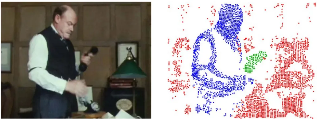
Consider Fig. 1(a). A basic task that one could expect a vision system to ac-complish is to detect the person in the image and to infer his shape or maybe other attributes. Contemporary person detectors achieve this goal by learning a classifier and a shape distribution from manually annotated training images. Is this annotation really necessary? Animals or infants are not supplied bounding boxes or segmented training images when they learn to see. Biological vision systems learn objects up to a certain degree of accuracy in an unsupervised way by making use of the natural ordering of the images they see [1]. Knowing that these systems exist, another objective of vision research must be to understand and emulate this capability.
A decisive step towards this goal is object-level segmentation in a purely bottom-up way. This step seems to be impossible given that such segmentation is ambiguous in the very most cases. In Fig. 1 the contrast between the white shirt and the black vest is much higher than the contrast between the vest and the background. How should a bottom-up method know that the shirt and the vest belong to the same object, while the background does not? The missing link This work was supported by the German Academic Exchange Service (DAAD) and
ONR MURI N00014-06-1-0734.
K. Daniilidis, P. Maragos, N. Paragios (Eds.): ECCV 2010, Part V, LNCS 6315, pp. 282–295, 2010. c
Fig. 1. Left: (a) Bottom-up segmentation from a single input frame is ambiguous.
Right: (b)Long term motion analysis provides important information for bottom-up object-level segmentation. Only motion information was used to separate the man and even the telephone receiver from the background.
can be established as soon as objects move1. Fig. 1 shows a good separation of
points on the person versus points on the background with the method proposed in this paper using only motion cues. As these clusters are consistently found for the whole video shot, this provides rich information about the person in various poses.
In this paper we describe a motion clustering method that can potentially be used for unsupervised learning. We argue that temporally consistent clusters over many frames can be obtained best by analyzing long term point trajectories rather than two-frame motion fields. In order to compute such trajectories, we run a tracker we developed in [2], which is based on large displacement optical flow [3]. It provides subpixel accurate tracks on one hand, and can deal with the large motion of limbs or the background on the other. Moreover, in contrast to traditional feature point trackers, it provides arbitrarily dense trajectories, so it allows to assign region labels far more densely. An alterative tracker that will probably work as well with our technique is the one from [4], though the missing treatment of large displacements might be a problem in some sequences.
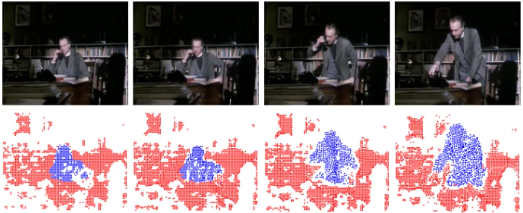
With these long term point trajectories at hand, we measure differences in how the points move. A key contribution of our method is that we define the distance between trajectories as the maximum difference of their motion over time. The person in Fig. 2 is sitting for a couple of seconds and then rising up. The first part of the shot will not provide any motion information to separate the person from the background. The most valuable cues are available at the point where the person moves fastest. A proper normalization further ensures that scenes with very large motion can be handled the same way as scenes with only little motion.
1Potentially even static objects can be separated if there is camera motion. In this
paper, however, we consider this case only as a side effect. Generally, active observers will be able to either move themselves or objects of interest in order to generate the necessary motion cues.
Fig. 2.Frames 0, 30, 50, 80 of a shot from Miss Marple: Murder at the vicarage. Up to frame 30, there is hardly any motion as the person is sitting. Most information is provided when the person is sitting up. This is exploited in the present approach. Due to long term tracking, the grouping information is also available at the first frames.
Given the pairwise distances between trajectories, we can build an affinity matrix for the whole shot and run spectral clustering on this affinity matrix [5,6]. Regarding the task as a single clustering problem, rather than deciding upon a single-frame basis, ensures that trajectories that belong to the same object but did not exist at the same time become connected by the transitivity of the graph. An explicit track repair as in [7] is not needed. Moreover, since we do not assume the number of clusters to be known in advance and the clusters should be spatially compact, we propose a spectral clustering method that includes a spatial regularity constraint allowing for model selection.
In order to facilitate progress in the field of object-level segmentation in videos, we provide an annotated dataset together with an evaluation tool, trajectories, and the binaries of our approach. This will allow for quantitative comparisons in the future. Currently the only reasonably sized dataset with annotation is the Hopkins dataset [8], which is specialized for factorization methods (sparse, manually corrected trajectories, all trajectories have the same length). The new dataset will extend the task to a more general setting where (1) the given tra-jectories are partially erroneous, (2) occlusion and disocclusion are a frequent phenomenon, (3) shots are generally larger, (4) density plays a role (it will be advantageous to augment the motion cues by static cues), and (5) the number of clusters is not known in advance.
2
Related Work
The fact that motion provides important information for grouping is well known and dates back to Koffka and Wertheimer suggesting the Gestalt principle of “common fate” [9]. Various approaches have been proposed for taking this group-ing principle into account. Difference images are the most simple way to let
temporally changing structures pop out. They are limited though, as they only indicate a local change but do not provide the reason for that change. This be-comes problematic if many or all objects in the scene are subject to a change (e.g. due to a moving camera). Much richer information is provided by opti-cal flow. Numerous motion segmentation methods based on two-frame optiopti-cal flow have been proposed [10,11,12,13]. The quality of these methods depends on picking a pair of frames with a clear motion difference between the objects. Some works have combined the flow analysis with the learning of an appearance model [14,15]. This leads to temporally consistent layers across multiple frames, but comes along with an increased number of mutually dependent variables. Rather than relying on optical flow, [16] estimates the motion of edges and uses those for a reasoning of motion layers.
In order to make most use of multiple frames and to obtain temporally con-sistent segments, a method should analyze trajectories over time. This is nicely exploited by multi-body factorization methods [17,18,19,20]. These methods are particularly well suited to distinguish the 3D motion of rigid objects by exploit-ing the properties of an affine camera model. On the other hand, they have two drawbacks: (1) factorization is generally quite sensitive to non-Gaussian noise, so few tracking errors can spoil the result; (2) it requires all trajectories to have the same length, so partial occlusion and disocclusion can actually not be han-dled. Recent works suggest ways to deal with these problems [19,20], but as the problems are inherent to factorization, this can only be successful up to a cer-tain degree. For instance, it is still required that a sufficiently large subset of trajectories exists for the whole time line of the shot.
There are a few works which analyze point trajectories outside the factor-ization setting [7,21,22,23]. Like the proposed method, these techniques do not require a dominant subset of trajectories covering the full time line, and apart from [21], which analyzes trajectories but runs the clustering on a single-frame basis, these methods provide temporally consistent clusters. Technically, how-ever, they are very different from our approach, with regard to the density of trajectories, how the distance between trajectories is defined, and in the algo-rithm used for clustering.
Trajectory clustering is not restricted to the domain of object segmentation. For instance, it has been used for learning traffic models in [24].
3
Point Tracking and Affinities between Trajectories
We obtain point trajectories by running the optical flow based tracker in [2] on a sequence. Fig. 3 demonstrates the most important properties of this tracker. Clearly, the coverage of the image by tracked points is much denser than with usual keypoint trackers. This is very advantageous for our task, as this allows us to assign labels far more densely than in previous approaches. Moreover, the denser coverage of trajectories will enable local reasoning from motion similari-ties as well as the introduction of spatial regularity constraints in the clustering method.Fig. 3. From left to right: Initial points in the first frame and tracked points in frame 211 and 400. Color indicates the age of the tracks. The scale goes from blue (young) over green, yellow, and red to magenta (oldest). The red points on the right person have been tracked since the person appeared behind the wall. The figure is best viewed in color.
Fig. 3 also reveals that points can be tracked over very long time intervals. A few points on the wall were tracked for all the 400 frames. The other tracks are younger because almost all points in this scene have become occluded. The person on the right appeared behind the wall and was initially quite far away from the camera. The initial points from that time have been tracked to the last frame and are visible as red spots among all the other tracks that were initialized later due to the scaling of the person.
Clearly, trajectories are asynchronous, i.e., they cover different temporal win-dows in a shot. This is especially true if the shot contains fast motion and large occluded areas. If we only selected the set of trajectories that survived the whole shot, this set would be very small or even empty and we would miss many dom-inant objects in the scene. So rather than picking a fully compatible subset, we define pairwise affinities between all trajectories that share at least one frame. The affinities define a graph upon which we run spectral clustering. Due to tran-sitivity, even tracks that do not share common frames can be linked up as long as there is a path in the graph that connects them.
According to the Gestalt principle of common fate, we should assign high affinities to pairs of points that move together. However, two persons walking next to each other share the same motion although they are different objects. We have to take into account that there are situations where we cannot tell two objects apart. The actual information is not in the common motion but in motion differences. As soon as one of the persons moves in another direction from the other one, we get a very clear signal that these two areas in the image do not belong together.
We define distances and affinities such that they best exploit this information. Regarding two trajectoriesAandB, we consider the instant, where the motion of the two points is most dissimilar:
d2(A, B) = maxtd2t(A, B). (1) Pairwise distances can only compare the compatibility of trajectories on the basis of translational motion models. To estimate the parameters of a more
general motion model, we would have to consider triplets or even larger groups of points, which is intractable. Another way is to estimate such models beforehand using a RANSAC procedure to deal with the fact that we do not know yet which points share the same motion model [7]. However, especially in case of many smaller regions, one needs many samples to ensure a set of points without outliers with high probability. Instead, we rely here on the fact that translational models are a good approximation for spatially close points and introduce a proper normalization in order to reduce the negative effects of this approximation.
We define the distance between two trajectories at a particular instanttas:
d2t(A, B) =dsp(A, B)
(uAt −uBt )2+ (
vtA−vtB)2
5σ2t . (2)
dsp(A, B) denotes the average spatial Euclidean distance of A and B in the
common time window. Multiplying with the spatial distance ensures that only proximate points can generate high affinities. Note that due to transitivity, points that are far apart can still be assigned to the same cluster even though their pairwise affinity is small.ut:=xt+5−xtandvt:=yt+5−ytdenote the motion
of a point aggregated over 5 frames. This averaging adds some further accuracy to the motion estimates. If less than 5 frames are covered we average over the frames that are available. Another important detail is the normalization of the distance by
σt= mina∈{A,B} 5
t=1
σ(xat+t, yta+t, t+t), (3) where σ : R3 → R denotes the local flow variation field. It can be considered a local version of the optical flow variance in each frame and is computed with linear diffusion where smoothing is reduced at discontinuities in the optical flow. The normalization by σt is very important to deal with both fast and slow motion. If there is hardly any motion in a scene, a motion difference of 2 pixels is a lot, whereas the same motion difference is negligible in a scene with fast motion. As scaling and rotation will cause small motion differences even locally, it is important to consider these differences in the context of the overall motion. Considering the local rather than the global variance of the optical flow makes a difference if at least three motion clusters appear in the scene. The motion difference between two of them could be small, while the other differences are large.
We use the standard exponential and a fixed scaleλ= 0.1 to turn the distances
d2(A, B) into affinities
w(A, B) = exp(−λd2(A, B)) (4) yielding an n×n affinity matrix W for the whole shot, where n is the total number of trajectories.
Fig. 4. From left to right, top to bottom: (a)Input frame.(b-h)The first 7 of
m = 13 eigenvectors. Clearly, the eigenvectors are not piecewise constant but show smooth transitions within the object regions. However, discontinuities in the eigenvec-tors correspond to object boundaries very well. This information needs to be exploited in the final clustering procedure.
4
Spectral Clustering with Spatial Regularity
Given an affinity matrix, the most common clustering techniques are agglomera-tive clustering, which runs a greedy strategy, and spectral clustering, which maps the points into a feature space where more traditional clustering algorithms like k-means can be employed. While the mapping in spectral clustering is a globally optimal step, the successive step that yields the final clusters is like all general clustering susceptible to local minima. We rely on the eigendecomposition of the normalized graph Laplacian to obtain the mapping and elaborate on deriv-ing good clusters from the resultderiv-ing eigenvectors. The settderiv-ing we propose also includes model selection, i.e., it decides on the optimum number of clusters.
LetDbe ann×ndiagonal matrix with entriesda=bw(a, b). The Laplacian eigenmap is obtained by an eigendecomposition of the normalized Laplacian
VΛV =D−12(D−W)D−12 (5)
and keeping the eigenvectors v0, ...,vm corresponding to the m+ 1 smallest
eigenvalues λ0, ..., λm. As λ0 = 0 and v0 is a constant vector, this pair can
be ignored. We choose m such that we keep all λ < 0.2. The exact choice of this threshold is not critical as long as it is not too low, since the actual model selection is done in eigenvector space. Sincemn, the eigendecomposition can be efficiently computed using the Lanczos method. We normalize all eigenvectors
vi to a range between 0 and 1.
In case of ideal data (distinct translational motion, no tracking errors), the mapping yieldsm=k−1 piecewise constant eigenvectors and thekclusters can be extracted by simple thresholding [5]. However, the eigenvectors are usually not that clean, as shown in Fig. 4. The eigenvectors typically show smooth transitions within a region and more or less clear edges between regions. Standard k-means
cannot properly deal with this setting either, since smooth transitions get ap-proximated by multiple constant functions, thus leading to an over-segmentation. At the same time the optimum number of clustersK is by no means obvious as clusters are represented by many eigenvectors.
As a remedy to both problems, we suggest minimizing an energy function that comprises a spatial regularity term. Letvai denote the ath component of theith eigenvector andva the vector composed of theath components of allm eigenvectors. Indexacorresponds to a distinct trajectory. LetN(a) be a set of neighboring trajectories based on the average spatial distance of trajectories. We seek to choose the total number of clustersKand the assignmentsπa∈ {1, ..., K} such that the following energy is minimized:
E(π, K) = a
K k=1
δπa,kva−μk2λ + ν a
b∈N(a)
1−δπa,πb
|va−vb|2 2
(6)
The first term is the unary cost that is minimized by k-means, where μk de-notes the centroid of cluster k. The norm · λ is defined as va −μλ =
i(via−μi)2/λi, i.e., each eigenvector is weighted by the inverse of the square root of its corresponding eigenvalue. This weighting is common in spectral clus-tering as eigenvectors that separate more distinct clusters correspond to smaller eigenvalues [25].
Clearly, if we do not restrictKor add a penalty for additional clusters, each tra-jectory will be assigned its own cluster and we will get a severe over-segmentation. The second term in (6) serves as a regularizer penalizing the spatial boundaries be-tween clusters. The penalty is weighted by the inverse differences of the eigenvec-tors along these boundaries. If there are clear discontinuities along the boundary of two clusters, the penalty for this boundary will be very small. In contrast, bound-aries within a smooth area are penalized far more heavily, which avoids splitting clusters at arbitrary locations due to smooth transitions in the eigenvectors. The parameterνsteers the tradeoff between the two terms. We obtain good results in various scenes by fixingν =1
2.
Minimizing (6) is problematic due to many local minima. We propose a heuris-tic that avoids such local minima. For a fixedK, we first run k-means with 10 random initializations. Additionally, we generate proposals by running hierarchi-cal 2-means clustering and selecting the 20 best solutions from the tree. We run k-means on these 20 proposals and select the best among all 30 proposals. Up to this point we consider only the first term in (6), since the proposals are gen-erated only according to this criterion. The idea is that for a large enoughKwe will get an over-segmentation that comprises roughly the boundaries of the true clusters. In a next step we consider merging moves. We successively consider the pair of clusters that when merged leads to the largest reduction of (6) including the second term. Merging is stopped if the energy cannot be further minimized. Finally, we run gradient descent to locally optimize the assignments. This last step mainly refines the assignments along boundaries. The whole procedure is run for allK∈ {1, ...,2m}and we pick the solution with the smallest energy.
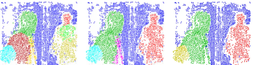
Fig. 5. Left: (a)Best k-means proposal obtained forK= 9. Over-segmentation due to smooth transitions in eigenvectors.Center: (b)Remaining 5 clusters after choosing the best merging proposals.Right: (c)Final segmentation after merging using affine motion models. Another cluster boundary that was due to the fast 3D rotation of the left person has been removed. The only remaining clusters are the background, the two persons, and the articulated arm of the left person.
Finally, we run a postprocessing step that merges clusters according to the mutual fit of their affine motion models. This postprocessing step is not abso-lutely necessary, but corrects a few over-segmentation errors. Fig. 5 shows the clusters obtained by k-means, after merging clusters of the k-means proposal, and after the postprocessing step.
5
Experimental Evaluation
5.1 Dataset and Evaluation Method
While qualitative examples often reveal more details of a method than pure numbers, scientific research always benefits from exact measurement. The task of motion segmentation currently lacks a compelling benchmark dataset to pro-duce such measurements and to compare among methods. While the Hopkins 155 dataset [8] has clearly boosted research in multi-body factorization, it is much too specialized for these types of methods, and particularly the checkerboard se-quences do not correspond to natural scenes. To this end, we have annotated 26 sequences, among them shots from detective stories and the 10 car and 2 people sequences from Hopkins 155, with a total of 189 annotated frames. The anno-tation is dense in space and sparse in time, with more frames being annotated at the beginning of a shot to allow also for the evaluation of methods that do not work well with long sequences. There are four evaluation modes. The first three expect the methods to be run only on the first 10, 50, and 200 frames, whereas for the last all available frames should be considered. It is planned to successively extend the dataset by more sequences to avoid over-fitting issues in the long run. An example of the annotation is shown in Fig. 6. This dataset is publicly available.
The evaluation tool yields 5 numbers for each sequence, which are then aver-aged across all sequences. The first number is thedensityof the points for which a cluster label is reported. Higher densities indicate more information extracted
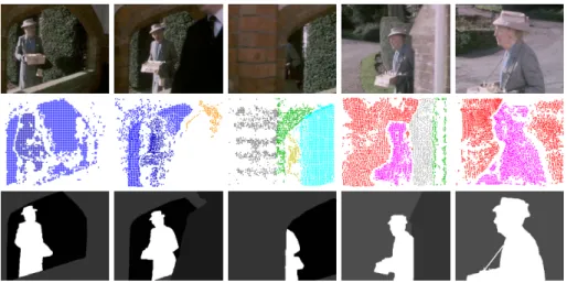
Fig. 6.Frames 1, 110, 135, 170, 250 of a shot fromMiss Marple: Murder at the vicarage
together with our clusters and the ground truth regions. There is much occlusion in this sequence as Miss Marple is occluded by the passing inspector and then by the building. Our approach can link tracks of partially occluded but not of totally occluded objects. A linkage of these clusters is likely to be possible based on the appearance of the clusters and possibly some dynamic model.
from the sequences and increase the risk of misclassifying pixels. The overall clustering erroris the number of bad labels over the total number of labels on a per-pixel basis. The tool optimally assigns clusters to ground truth regions. Multiple clusters can be assigned to the same region to avoid high penalties for over-segmentations that actually make sense. For instance, the head of a person could be detected as a separate cluster even though only the whole person is annotated in the dataset. All points covering their assigned region are counted as good labels, all others count as bad labels. In some sequences, objects are marked that are easy to confuse due to their size or very little motion infor-mation. A penalty matrix defined for each sequence assigns smaller penalty to such confusions. Theaverage clustering error is similar to the overall error but averages across regions after computing the error for each region separately. Usually the average error is much higher than the overall error, since smaller objects are more difficult to detect, confused regions always pay the full penalty, and not covering an object yields a 100% error for that region.
Since the above evaluation method allows for cheating by producing a severe over-segmentation, we also report theover-segmentation error, i.e., the num-ber of clusters merged to fit the ground truth regions. Methods reporting good numbers with a very high over-segmentation error should be considered with care.
As the actual motivation for motion segmentation is the unsupervised extrac-tion of objects, we finally report the number of regions covered with less than 10% error. One region is subtracted per sequence to account for the background.
tracks time our method 15486 497s
GPCA 12060 2963s
LSA 12060 38614s
RANSAC 12060 15s
ALC 957 22837s
[19], which can deal with either incomplete or corrupted trajectories (ALC). When running these methods, we use the same trajectories as for our own method. Except for ALC with in-complete tracks, all these techniques require the tracks to have full length, so we restrict the available set of tracks accordingly. For this reason, the density with these methods is
con-siderably smaller, especially when more frames are taken into account and the areas of occlusion and disocclusion grow bigger. Moreover, all these methods ask for the number of regions to be given in advance. We give them the correct num-ber, whereas we select the model in our approach automatically. Since ALC gets intractably slow when considering more than 1000 trajectories (see Table 1), we randomly subsampled the tracks for this method by a factor 16. In Table 2 we multiply the density again by this factor to make the results comparable.
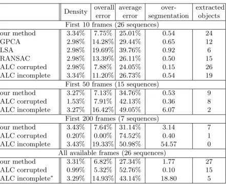
Table 2.Evaluation results. The sequence marple7 was ignored in the entry marked with∗as the computation took more than 800 hours.
Density overall average over- extracted error error segmentation objects First 10 frames (26 sequences)
our method 3.34% 7.75% 25.01% 0.54 24
GPCA 2.98% 14.28% 29.44% 0.65 12
LSA 2.98% 19.69% 39.76% 0.92 6
RANSAC 2.98% 13.39% 26.11% 0.50 15
ALC corrupted 2.98% 7.88% 24.05% 0.15 26 ALC incomplete 3.34% 11.20% 26.73% 0.54 19
First 50 frames (15 sequences)
our method 3.27% 7.13% 34.76% 0.53 9 ALC corrupted 1.53% 7.91% 42.13% 0.36 8 ALC incomplete 3.27% 16.42% 49.05% 6.07 2
First 200 frames (7 sequences)
our method 3.43% 7.64% 31.14% 3.14 7 ALC corrupted 0.20% 0.00% 74.52% 0.40 1 ALC incomplete 3.43% 19.33% 50.98% 54.57 0
All available frames (26 sequences)
our method 3.31% 6.82% 27.34% 1.77 27 ALC corrupted 0.99% 5.32% 52.76% 0.10 15 ALC incomplete∗ 3.29% 14.93% 43.14% 18.80 5
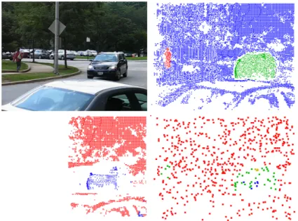
Fig. 7. From left to right: (a)Frame 40 of the cars4 sequence from the Hopkins dataset.(b)The proposed method densely covers the image and extracts both the car and the person correctly.(c)RANSAC (like all traditional factorization methods) can assign labels only to complete tracks. Thus large parts of the image are not covered.
(d)ALC with incomplete trajectories [19] densely covers the image, but has problems assigning the right labels.
Clearly, the more traditional methods like GPCA, LSA, and RANSAC do not perform well on this dataset (which comprises a considerable number of sequences from the Hopkins dataset). Even when considering only 10 frames, i.e. there is only little occlusion, the error is much larger than for the proposed approach. The 10-frame result for ALC with a correction for corrupted tracks is quite good and comparable to ours with some advantages with regard to over-segmentation and extracted objects. This is mainly due to the correct number of regions given to ALC.
As the number of frames is increased, the density of ALC decreases and its performance goes down. With more occlusions, ALC with incomplete tracks be-comes interesting, as it is the only method in this comparison apart from ours that can exploit all trajectories. However, its ability to handle sparse trajectories is limited. ALC still needs a sufficiently large set of complete tracks in order to extrapolate the missing entries, whereas the approach described in this paper just requires some overlapping pieces of trajectories to cluster them together. We see a larger over-segmentation error for the longer sequences, as occlusion intro-duces ambiguities and makes the clustering problem generally harder, but at the same time we obtain more information about the tracked objects. Moreover, by considering more frames, objects that were static in the first frames can be
the whole image with labels, but as this is achieved by extrapolating missing entries, lots of errors occur. In case ALC cannot find the given number of regions, it uses an MDL criterion, which leads to a very high over-segmentation error.
The density of our approach is still far from 100%. This is mainly due to efficiency considerations, as the tracker in [2] could also produce denser trajec-tories. However, the trajectories already cover the image domain without too many larger gaps. In this paper, we did without static cues to keep the pa-per uncluttered. Given these point labels, however, it actually should be quite straightforward to obtain a dense segmentation by considering color or boundary information.
6
Conclusions
We have presented a technique for object-level segmentation in a pure bottom-up fashion by exploiting long term motion cues. Motion information is aggregated over the whole shot to assign labels also to objects that are static in a large part of the sequence. Occlusion and disocclusion is naturally handled by this approach, which allows to gather information about an object from multiple aspects. This kind of motion segmentation is far more general than most previous techniques based on two-frame optical flow or a sparse subset of complete trajectories. We believe that such a general setting is very relevant, as it will ultimately enable unsupervised learning of objects from appropriate video data. We hope that by providing a benchmark dataset that comprises a variety of easier and harder sequences, we can foster progress in this field.
References
1. Spelke, E.: Principles of object perception. Cognitive Science 14, 29–56 (1990) 2. Sundaram, N., Brox, T., Keutzer, K.: Dense point trajectories by GPU-accelerated
large displacement optical flow. In: European Conf. on Computer Vision. LNCS, Springer, Heidelberg (2010)
3. Brox, T., Malik, J.: Large displacement optical flow: descriptor matching in vari-ational motion estimation. IEEE Transactions on Pattern Analysis and Machine Intelligence (to appear)
4. Sand, P., Teller, S.: Particle video: long-range motion estimation using point tra-jectories. International Journal of Computer Vision 80, 72–91 (2008)
5. Shi, J., Malik, J.: Normalized cuts and image segmentation. IEEE Transactions on Pattern Analysis and Machine Intelligence 22, 888–905 (2000)
6. Ng, A.Y., Jordan, M.I., Weiss, Y.: On spectral clustering: Analysis and an algo-rithm. In: Advances in Neural Information Processing Systems (2002)
7. Sivic, J., Schaffalitzky, F., Zisserman, A.: Object level grouping for video shots. International Journal of Computer Vision 67, 189–210 (2006)
8. Tron, R., Vidal, R.: A benchmark for the comparison of 3-D motion segmentation algorithms. In: Int. Conf. on Computer Vision and Pattern Recognition (2007) 9. Koffka, K.: Principles of Gestalt Psychology. Hartcourt Brace Jovanovich, New
York (1935)
10. Wang, J.Y.A., Adelson, E.H.: Representing moving images with layers. IEEE Transactions on Image Processing 3, 625–638 (1994)
11. Weiss, Y.: Smoothness in layers: motion segmentation using nonparametric mixture estimation. In: Int. Conf. on Computer Vision and Pattern Recognition, pp. 520– 527 (1997)
12. Shi, J., Malik, J.: Motion segmentation and tracking using normalized cuts. In: Proc. 6th International Conference on Computer Vision, Bombay, India, pp. 1154– 1160 (1998)
13. Cremers, D., Soatto, S.: Motion competition: A variational framework for piecewise parametric motion segmentation. International Journal of Computer Vision 62, 249–265 (2005)
14. Xiao, J., Shah, M.: Motion layer extraction in the presence of occlusion using graph cuts. IEEE Transactions on Pattern Analysis and Machine Intelligence 27, 1644–1659 (2005)
15. Pawan Kumar, M., Torr, P., Zisserman, A.: Learning layered motion segmentations of video. International Journal of Computer Vision 76, 301–319 (2008)
16. Smith, P., Drummond, T., Cipolla, R.: Layered motion segmentation and depth ordering by tracking edges. IEEE Transactions on Pattern Analysis and Machine Intelligence 26, 479–494 (2004)
17. Costeira, J., Kanande, T.: A multi-body factorization method for motion analysis. In: Int. Conf. on Computer Vision, pp. 1071–1076 (1995)
18. Yan, J., Pollefeys, M.: A general framework for motion segmentation: indepen-dent, articulated, rigid, non-rigid, degenerate and non-degenerate. In: Leonardis, A., Bischof, H., Pinz, A. (eds.) ECCV 2006. LNCS, vol. 3954, pp. 94–106. Springer, Heidelberg (2006)
19. Rao, S.R., Tron, R., Vidal, R., Ma, Y.: Motion segmentation via robust subspace separation in the presence of outlying, incomplete, or corrupted trajectories. In: Int. Conf. on Computer Vision and Pattern Recognition (2008)
20. Elhamifar, E., Vidal, R.: Sparse subspace clustering. In: Int. Conf. on Computer Vision and Pattern Recognition (2009)
21. Brostow, G., Cipolla, R.: Unsupervised Bayesian detection of independent motion in crowds. In: Int. Conf. on Computer Vision and Pattern Recognition (2006) 22. Cheriyadat, A., Radke, R.: Non-negative matrix factorization of partial track data
for motion segmentation. In: Int. Conf. on Computer Vision (2009)
23. Fradet, M., Robert, P., P´erez, P.: Clustering point trajectories with various life-spans. In: Proc. European Conference on Visual Media Production (2009) 24. Wang, X., Tieu, K., Grimson, E.: Learning semantic scene models by
trajec-tory analysis. In: Leonardis, A., Bischof, H., Pinz, A. (eds.) ECCV 2006. LNCS, vol. 3953, pp. 110–123. Springer, Heidelberg (2006)
25. Belongie, S., Malik, J.: Finding boundaries in natural images: A new method using point descriptors and area completion. In: Burkhardt, H.-J., Neumann, B. (eds.) ECCV 1998. LNCS, vol. 1406, pp. 751–766. Springer, Heidelberg (1998)