Carmichael_unc_0153D_18458.pdf

PROBABILISTIC AND GEOMETRIC APPROACHES TO THE ANALYSIS OF NON-STANDARD

DATA

Iain Carmichael

A dissertation submitted to the faculty of the University of North Carolina at Chapel Hill in

partial fulfillment of the requirements for the degree of Doctor of Philosophy in the

Department of Statistics and Operations Research.

Chapel Hill

2019

ABSTRACT

Iain Carmichael: Probabilistic and geometric approaches to the analysis of non-standard data

(Under the direction of: Shankar Bhamidi and J.S Marron)

This dissertation explores topics in machine learning, network analysis, and the foundations of

statistics using tools from geometry, probability and optimization.

The rise of machine learning has brought powerful new (and old) algorithms for data analysis. Much

of classical statistics research is about understanding how statistical algorithms behave depending on

various aspects of the data. The first part of this dissertation examines the

support vector machine

clas-sifier (SVM). Leveraging Karush-Kuhn-Tucker conditions we find surprising connections between SVM

and several other simple classifiers. We use these connections to explain SVM’s behavior in a variety of

data scenarios and demonstrate how these insights are directly relevant to the data analyst.

The next part of this dissertation studies networks which evolve over time. We first develop a method

to empirically evaluate vertex centrality metrics in an evolving network. We then apply this methodology

to investigate the role of

precedent

in the US legal system.

Next, we shift to a probabilistic perspective on temporally evolving networks. We study a general

probabilistic model of an evolving network that undergoes an abrupt change in its evolution dynamics.

In particular, we examine the effect of such a change on the network’s structural properties. We develop

mathematical techniques using

continuous time branching processes

to derive quantitative error bounds

for functionals of a major class of these models about their large network limits. Using these results,

we develop general theory to understand the role of abrupt changes in the evolution dynamics of these

models. Based on this theory we derive a consistent, non-parametric

change point detection

estimator.

ACKNOWLEDGEMENTS

I owe an enormous amount of gratitude to my two advisors, Shankar Bhamidi and Steve Marron,

for their enthusiasm, support and encouragement over the past five years. I suspect I went down some

unorthodox paths during my PhD and they always supported these forays – or at least the worthwhile

ones.

I thank Sayan Banerjee and Jan Hannig for their collaboration (and patience) on research projects

over the years. I am appreciative of Andrew Nobel and Quoc Tran-Dinh for serving on my committee

and always being willing to chat about both technical and career problems in statistics. I am grateful

to everyone

who helped me create STOR 390 and turn it into a permanent part of the statistics

cur-riculum, particularly Brendan Brown, Shankar Bhamidi, Robin Cunningham, Mario Giacomazzo, Dylan

Glotzer, Varun Goel and Marshall Markham. I am grateful to Christine Keat, Alison Kieber and Samantha

Radel, and for helping me to navigate UNC so smoothly. I am thankful for all the support I received from

other graduates students including, Kelly Bodwin, Eric Friedlander, Jimmy Jin, Meilei Jung, John

Palow-itch, Zhengling Qi, and James Wilson. I am especially grateful to Jonathan Williams for his (grudging)

willingness to engage in hours (at this point days) of discussions and debates about statistics.

Part of what I love about statistics is how one can parachute into another discipline and work closely

with talented and passionate collaborators. I thank CourtListener, Michael Lissner, and James Wudel

for teaching me more about the law and providing access to a wealth of legal data. I am grateful to Ben

Calhoun, Joseph Geradts, Katherine Hoadley, Linnea Olsen, Charles Perou, and Melissa Troester.

for teaching me about breast cancer pathology and genetics. I thank Heather Couture and Marc

Ni-ethammer for introducing me to medical imaging. I am appreciative of Ryan Thornburg for teaching

me about journalism in the digital era. I thank Matt Barr, Cameron Freer and Ben Vigoda for everything

I learned during my internship at Gamalon. I thank Yiming Hu, Yunxiao Liu, and John Palowitch for

being awesome teammates for Citadel’s data science competitions. I am appreciative of my

uate students and their hard work: Kate Cho, Scott Garcia, James Jushchuk, Michael Kim, Ethan Koch

and Charles Tang. I sincerely thank Sandeep Sarangi for his timely and continuous support on UNC’s

computing cluster without which my productivity would have been cut in half.

TABLE OF CONTENTS

LIST OF TABLES . . . xiii

LIST OF FIGURES . . . xiv

LIST OF ABBREVIATIONS AND SYMBOLS . . . xvii

1

Introduction . . . .

1

1.1

Support vector machine . . . .

2

1.2

Network analysis and the law . . . .

3

1.3

Dynamic network models and change point detection . . . .

4

1.4

False confidence . . . .

5

1.5

Data science . . . .

6

1.6

Statistical software . . . .

6

1.7

Teaching and undergraduate mentorship . . . .

7

2

Linear classifiers . . . .

9

2.1

Mean Difference . . . 10

2.2

Naive Bayes, linear discriminant analysis, and maximal data piling. . . 10

2.3

Data transformation perspective: covariance matrix + mean difference . . . 13

2.4

Linear discriminant vs. maximal data piling. . . 15

3

Geometric Insights into Support Vector Machine Behavior using the KKT Conditions . . . 20

3.1

Introduction . . . 20

3.1.1

Motivating Example . . . 21

3.1.2

Related Literature . . . 24

3.2

Setup and Notation . . . 26

3.2.2

Data Transformation . . . 27

3.2.3

Maximal Data Piling Direction . . . 28

3.2.4

Support Vector Machine . . . 29

3.3

Hard Margin SVM in High Dimensions . . . 30

3.3.1

Complete Data Piling Geometry . . . 30

3.3.2

Hard Margin SVM and Complete Data Piling . . . 31

3.3.3

Hard Margin KKT Conditions . . . 32

3.3.4

Proofs for Hard Margin SVM . . . 33

3.4

Soft Margin SVM Small and Large

C

Regimes. . . 34

3.4.1

Soft Margin SVM KKT Conditions . . . 36

3.4.2

Proofs for Small

C

Regime . . . 38

3.4.3

Proofs for Large

C

Regime . . . 41

3.5

Summary of SVM Regimes . . . 41

3.5.1

Small

C

Regime and the Mean Difference . . . 42

3.5.2

Class Imbalance and the MD Regime . . . 43

3.5.3

Small

C

Regime and Margin Bounce . . . 43

3.5.4

Large

C

Regime and the Hard-Margin SVM . . . 44

3.5.5

Hard-Margin SVM and the (cropped) Maximal Data Piling Direction . . . 44

3.6

Applications of SVM Regimes . . . 45

3.6.1

Tuning SVM via Cross-Validation . . . 46

3.6.2

Improved SVM Intercept for Cross-Validation . . . 48

3.7

Discussion . . . 50

3.7.1

Geometry of Complete Data Piling . . . 50

3.7.2

nu-SVM and the Reduced Convex Hull . . . 51

3.7.3

Relations Between SVM and Other Classifiers . . . 52

4

Vertex Centrality Metrics . . . 59

4.2

Sort experiment methodology . . . 60

4.2.1

Discussion . . . 61

5

Vertex Centrality Metrics with Applications to the Law . . . 64

5.1

Introduction . . . 64

5.2

Precedent and case law citation network research . . . 69

5.3

Methods . . . 71

5.3.1

Vertex Centrality Metrics . . . 71

5.3.2

The methodology . . . 73

5.3.2.1

Sort experiment . . . 74

5.3.2.2

Motivation and interpretation of the methodology . . . 75

5.3.3

Data . . . 75

5.4

Results . . . 77

5.4.1

Supreme Court results . . . 77

5.4.1.1

Time agnostic metrics . . . 77

5.4.1.2

Time aware metrics . . . 81

5.4.2

Federal Appellate Results . . . 84

5.5

Discussion . . . 85

5.5.1

Out-degree beats in-degree . . . 85

5.5.1.1

Preferential attachment . . . 85

5.5.1.2

Case qualities possibly driving out-degree . . . 86

5.5.2

Time awareness improves prediction of future citations . . . 89

5.5.3

PageRank and questions of first impression . . . 90

5.5.4

Deciding which vertex centrality metric to use . . . 92

5.6

Conclusion . . . 94

6

Fluctuation bounds for continuous time branching processes and nonparametric

change point detection in growing networks . . . 95

6.1

Introduction . . . 95

6.1.2

Informal description of our aims and results . . . 96

6.1.3

Model definition . . . 97

6.1.4

Organization of the paper . . . 98

6.2

Preliminaries . . . 98

6.2.1

Mathematical notation . . . 98

6.2.2

Assumptions on attachment functions . . . 99

6.2.3

Branching processes . . . 100

6.3

Main Results . . . 101

6.3.1

Convergence rates for model without change point . . . 101

6.3.2

Change point detection: Sup-norm convergence of degree distribution

for the standard model . . . 104

6.3.3

Multiple change points . . . 107

6.3.4

The quick big bang model . . . 108

6.3.5

Change point detection. . . 110

6.4

Discussion . . . 111

6.5

Initial embeddings and constructions . . . 114

6.5.1

Road map for proofs of the main results . . . 114

6.5.2

Initial constructions . . . 115

6.6

Change point model for fixed time

a: point-wise convergence for general characteristics . . . 119

6.6.1

Notation . . . 119

6.6.2

Definitions . . . 120

6.6.3

Proof of Theorem 6.6.1: . . . 121

6.7

Proofs: Sup-norm convergence of degree distribution for the standard model . . . 129

6.7.1

Proof of Theorems 6.3.6 and 6.3.9 . . . 129

6.7.1.1

Notation . . . 130

6.7.2

Proof of Corollary 6.3.11: . . . 142

6.8

Proofs: Quick Big bang . . . 143

6.8.2

Proof of Theorem 6.3.16: . . . 158

6.9

Proofs: Convergence rates for model without change point . . . 164

6.10 Proofs: Change point detection . . . 176

7

An exposition of the false confidence theorem . . . 180

7.1

Introduction . . . 180

7.2

Main ideas . . . 182

7.3

Uniform with Jeffreys’ prior . . . 183

7.4

Marginal posterior from two uniform distributions . . . 186

7.5

Marginal posterior from two Gaussian distributions . . . 187

7.6

Concluding remarks and future work . . . 190

7.7

Acknowledgments . . . 190

8

Data science vs. statistics: two cultures? . . . 191

8.1

Introduction . . . 191

8.2

What is Data Science. . . 193

8.2.1

What’s in a Name? . . . 195

8.2.2

Critiques of Statistics . . . 196

8.2.3

Reproducibility and Communication . . . 198

8.3

Modes of Variation . . . 199

8.3.1

Prediction vs. Inference (Do vs. Understand) . . . 200

8.3.2

Empirically vs. Theoretically driven . . . 201

8.3.3

Problem First vs. Hammer Looking for a Nail . . . 202

8.3.4

The 80/20 Rule . . . 202

8.4

Going Forward . . . 203

8.4.1

Research . . . 203

8.4.1.1

Complex Data and Representation. . . 203

8.4.1.2

Robustness to Unknown Heterogeneity . . . 204

8.4.1.4

Automation and Interpretability . . . 205

8.4.1.5

Machine Learning and Data Processing . . . 206

8.4.2

Computation and Communication. . . 207

8.4.2.1

Literate Programming . . . 207

8.4.2.2

Open Source . . . 209

8.4.3

Education . . . 210

8.4.3.1

More Computation . . . 211

8.4.3.2

Pedagogy . . . 212

8.5

Conclusion . . . 213

APPENDIX: ADDITIONAL VERTEX CENTRALITY METRICS DETAILS . . . 214

LIST OF TABLES

5.5.1 This table shows the top ten cases by out-degree for the Supreme Court and

in the Federal Appellate network. Nine of the top ten cases as ranked by

LIST OF FIGURES

3.1.1 SVM reduces to another classifier under the condition stated in the arrow. Solid

line means the relation always holds. Dashed line means the relation may or

may not hold depending on the data. For example, SVM reduces to the mean

difference when the classes are balanced and

C

is sufficiently small (C

≤

C

)

which is shown in Theorem 3.4.5. . . 22

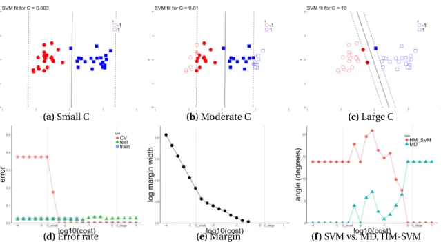
3.1.2 (Balanced classes) The top rows show the SVM fit for various values of

C

. The

bottom row shows diagnostics which are described in the text. Figure 3.1.2d

shows that the cross-validation error curve can be very different from the

train-ing and test error. Figure 3.1.2f shows that for small enough values of

C

, the

SVM and MD directions are the same. . . 23

3.1.3 (Unbalanced classes). The panels are the same as in Figure 3.1.2, but the data

now have one additional point added. When

C

is small, the top left panel

shows SVM classifies every point to the larger class (the separating hyperplane

is pushed past the smaller class). For this unbalanced example the

cross-validation, train and test error all behave similarly, unlike the balanced case

(compare Figure 3.1.3d to 3.1.2d). When

C

is small, the angle between SVM

and the MD is small but not exactly zero (compare Figure 3.1.3f to 3.1.2f). . . 23

3.6.1 Tuning error curves for standard SVM intercept vs. improved SVM intercept. . . 49

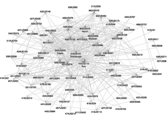
5.1.1 A visual of a network; this plot shows Roe v. Wade and its neighboring cases.

Each dot represents a case and each gray arrow represents a citation from one

case to another. This graphic is reproduced from (Fowler et al.,

2007). . . 66

5.1.2 A simple example of a citation network with six cases. The highlighted case A

has been cited three times. Therefore, case A has an in-degree equal to three.

Similarly, case A cites two cases and therefore has an out-degree equal to two. . . 67

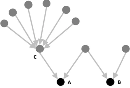
5.3.1 This Figure shows a small citation network. Cases A and B would be ranked

equally by in-degree, but case A would be ranked better by eigenvector

central-ity metrics as described in text above. . . 72

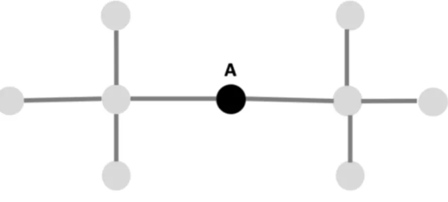
5.3.2 This Figure shows a simple network. The highlighted node A would be ranked

highest by most positional vertex centrality metrics since it is “closest" to all

other nodes. The network is undirected here for simplicity. . . 73

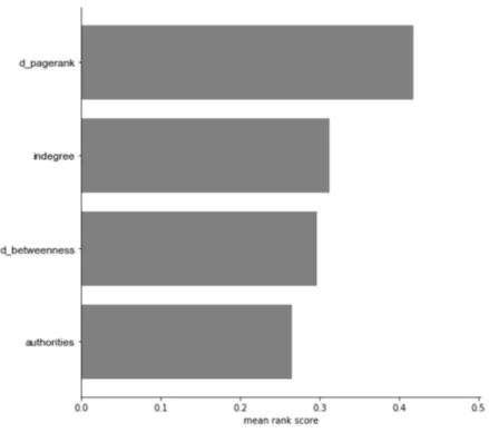
5.4.1 Authorities performs better than the three other in-degree based centrality metrics. . . 78

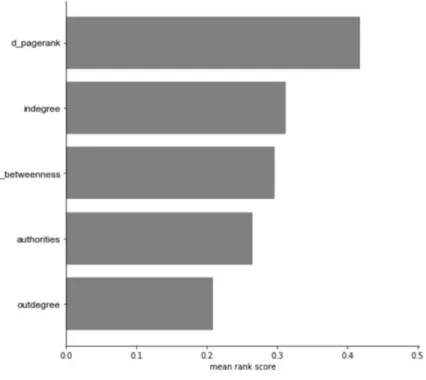
5.4.2 Figure 5.4.2 is the same as Figure 5.4.1 with the addition of out-degree.

Out-degree outperforms in-Out-degree and other more sophisticated vertex centrality

5.4.3 This figure shows a scatter plot of opinion text length and out-degree for all

Supreme Court cases. The plot includes the linear model fit of out-degree

ver-sus number of words (R

=

0.36, p-value

<

10

). Note that outliers were first

removed by removing the top 1% longest cases and top 1% highest out-degree

cases. The linear model found a significant relationship at an alpha level of

0.05. The conclusion is that opinion text length and out-degree are related. . . 80

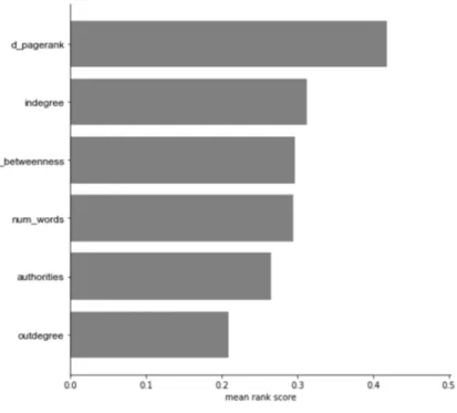
5.4.4 Text length, measured by the number of words contained in the court opinion,

does better than in-degree in the sort experiment by a small but statistically

significant amount. . . 81

5.4.5 Histogram of citation ages i.e. the difference between the date of the citing

opinion and the cited

opinion. The Supreme Court generally favors citing

re-cent cases over older cases. . . 82

5.4.6 Results of the sort experiment for both time-aware and time-agnostic metrics.

Various centrality metrics are on the y-axis and the mean rank score is on the

x-axis. Generally, time aware metrics perform better than the time-agnostic metrics. . . 83

5.4.7 Y-axis is vertex centrality metrics and x-axis is mean rank score. Results of

the sort experiment for metrics performed on the Federal Appellate courts:

in-degree now does better than both out-in-degree and authorities. Out-in-degree beats

authorities. Hubs now does worse than in-degree. . . 84

5.5.1 This figure shows the median in-degree and out-degree of Supreme Court cases

by year. The Warren Court, which lasted from 1953 to 1969, is visible in the dip

in in-degree, out-degree, and case length. Median was selected instead of mean

because median is more robust to outliers. . . 88

5.5.2 PageRank is biased to favor older cases. This is a plot of each case’s PageRank

value versus the year that case occurs. . . 91

6.3.1 The function

d

(

·

). Here

n

=

2

∗

10

,

γ

=

0.5,

f

(i

)

=

i

+

2,

f

(i

)

=

p

i

+

2,

h

=

log log

n,

b

=

n

. (A) The vertical, red line shows the true change

point. The vertical, blue, dashed line shows the estimated change point. The

horizontal, dashed, blue line shows the threshold value

b

. (B) The black curve

shows the mean of

d

(

·

) and the grey, curved region shows the 10/90t h

per-centiles (computed from 100 simulations). The blue, vertical region shows

10/90t h

percentiles of the estimated change point. . . 111

7.2.1 A sample of realizations from the sampling distribution of the posterior density

of the mean,

θ

, for Gaussian data with known variance and normal prior on

θ

.

7.3.1 The leftmost panel is a plot of the sampling probability,

p, as a function of

ε

, as

given by equation (7.3.2), for

α

=

.5. The center and rightmost panels are

ran-domly observed realizations of the posterior density of

θ

, with a .3-ball around

θ

represented by the shaded green regions. In all panels, the true parameter

value is set at

θ

=

1. . . 185

7.4.1 The leftmost panel is a plot of the estimated sampling probability,

p

b

, as a

func-tion of

ε

, as given by equation (7.4.1), for

α

=

.5. The center and rightmost

panels are randomly observed realizations of the posterior density of

Ψ

, with

a 6-ball around

ψ

represented by the shaded green regions. In all panels, the

true parameter value is set at

ψ

=

10. . . 187

7.5.1 Each panel is a plot of the estimated sampling probability of

p, as a function

of

ε

, using the posterior density equation (7.5.1), and setting

α

=

.5. The true

parameter value is

ψ

=

10. . . 189

7.5.2 Each panel is a plot of the estimated sampling probability of

p, as a function

of

ε

, using the posterior density equation (7.5.1), and setting

α

=

.05. The true

parameter value is

ψ

=

10. . . 189

7.5.3 Each panel exhibits randomly observed realizations of the posterior density of

ψ, equation (7.5.1), with a 4-ball around

ψ

=

10 represented by the shaded

green regions. . . 190

8.5.1 Results of sort experiment for PageRank and Hubs on a reversed graph

com-pared to previous metrics. Hubs performed the best among these metrics and

LIST OF ABBREVIATIONS AND SYMBOLS

CTBP

|| · ||

DAG

FCT

FLD

MD

MDP

PCA

R

RCH

SVM

Continuous time branching processes

Euclidean norm (unless stated otherwise)

Directed acyclic graph

CHAPTER 1

Introduction

One of the major changes in statistics over the past couple decades is the upswing in the use of

com-plex algorithms for data analysis. Classical statistical algorithms such as linear regression and principal

components analysis (PCA) can be understood through straightforward linear algebra and geometric

considerations. Modern statistical algorithms such as neural networks do not have such simple

math-ematical characterizations. This raises theoretical, computational and practical challenges for data

an-alysts. One of the aims of my research is to uncover some of the simple, mathematical concepts which

underly some of these more sophisticated algorithms. To this end, Chapter 3 of this dissertation presents

new geometric insights into the

support vector machine

(SVM) classifier.

Another shift in modern data analysis is the rise of non-standard data such as networks, text and

images. These kinds of data often demand new theoretical and methodological tools. For example,

the explosion of network data – particularly networks which evolve over time– has given rise to many

new mathematical models and statistical methods (e.g. community detection and vertex centrality

met-rics). Due to the complex statistical dependencies in these network models, it is difficult to understand

their properties. Another aim of my research is to develop mathematical and statistical tools which can

be used to rigorously analyze the properties of statistical network algorithms. To this end,Chapter 5

presents new statistical methodology to empirically evaluate vertex centrality metrics in a dynamic

net-work. Chapter 6 presents new theory for dynamic network models and network change point detection

algorithms.

Finally, these recent changes in statistics have ignited new – and reignited old– debates

about the foundations of statistics.

This includes topics such as reproducibility, the roles of

ex-ploratory/predictive/confirmatory analyses and statistical frameworks such as Bayesian, Frequentist

and Fiducial inference. We explore several of these topics in Chapters 7 and 8.

a few simple ideas can be used to understand a large number of classification algorithms. Chapter 4

gives a brief overview of the statistical methodology that is developed in Chapter 5. Sections 1.6 and 1.7

discuss the software and educational contributions made during the development of this dissertation.

The other sections provide a summary of these projects.

1.1 Support vector machine

Chapter 3 studies the

support vector machine

classifier (SVM) and provides new mathematical

expla-nations of SVM’s behavior on real data as well as demonstrating connections between SVM and a variety

of other classifiers (see Figure 3.1.1). This project started because Prof. Marron noticed that

occasion-ally the SVM

normal vector

direction points in the same direction as the

mean difference

(MD) normal

vector and asked me to figure out when this happens. I found this observation surprising because the

SVM optimization is a quadratic program and in general does not have an analytic solution. I therefore

(naively) tried to prove that SVM could

not

give exactly the MD direction, except for perhaps in very

special data scenarios. I ended up proving the opposite. For soft-margin SVM on a binary classification

dataset, this MD like behavior

always

happens

when the two classes are balanced; when the classes are

unbalanced, the MD like behavior occurs approximately (see Theorem 3.4.5).

SVM does not have an analytical solution in general so reasoning about how the SVM solution

de-pends on the data is challenging. For example, when tuning soft-margin SVM it is very easy to make

SVM classify every data point into one class (see Section 3.1.1). Even worse, when using cross-validation

to tune SVM, sometimes the cross-validation error curve looks significantly different from the test error

curve (see Figure 3.1.3d). Using the Karush-Kuhn-Tucker conditions we are able to provide rigorous

ex-planations of each of these phenomena. These mathematical exex-planations provide further insight into a

variety of other SVM phenomena, for example, how SVM cross-validation can be sensitive to properties

of the data (see Section 3.6) and connections between SVM (both hard and soft margin) and other

clas-sifiers such as naive Bayes, Fisher’s linear discriminant and the maximal data piling direction (see Figure

3.1.1).

1_{The MD is perhaps the most simple linear classifier for binary classes; compute each class mean and let the normal vector} point from one mean to the other. The MD classifier is discussed in more detail in Chapter 2.

This project is joint work with Prof. Marron and is under review for publication at the time of this

writing (Carmichael and Marron,

2017).

1.2 Network analysis and the law

When the Supreme Court of the United States decides a case, the judges write an opinion. In the

US (and many other countries) these court opinions are new law. Like academic articles, these opinions

cite one another and create the Supreme Court citation network. A fundamental part of the US legal

system is that judges must use previous legal decisions to decide new cases. In other words, judges are

bound by

precedent. Studying the Supreme Court citation network, or the much larger citation network

of all US legal opinions, provides insights into how the law evolves over time. In (Carmichael et al.,

2017),

reproduced in Chapter 5, we use

vertex centrality metrics

to study the influence of precedent in the US

Supreme Court and Federal Appellate circuit.

To obtain this legal citation network data

, we partnered with a legal non-profit, Courtlistener

which provides access to about 3 million US legal cases including the text of the opinion, the citation

network and a variety of other data.

In (Carmichael et al.,

2017), we find new, empirical evidence of the role that precedent plays in the

Supreme Court and US Federal appellate court. These findings come from a new methodology we

de-velop to evaluate different vertex centrality metrics in an evolving network. In particular, we make the

surprising discovery that an opinion’s out-degree

(and related metrics) is more predictive of that

opin-ion receiving future citatopin-ions than the opinopin-ion’s in-degree. In other words, the length of an opinopin-ion’s

bibliography, from a network standpoint, is a better measure of a case’s popularity than the number of

citations that case has already received. This fact is surprising due to the popularity of mathematical

network models such as

preferential attachment

(Barabási and Albert,

1999) where the current number

of citations plays a fundamental role in acquiring future citations. From a legal scholarship standpoint,

4_{https://www.courtlistener.com/}

however, this finding is interesting because it speaks to the importance of

precedent

in the Supreme

Court (and broader legal system).

The methodology we develop to empirically evaluate vertex centrality metrics, which we call the

“sort experiment", is of independent interest for network science and information retrieval. Because

the focus of (Carmichael et al.,

2017) is on the legal application, Chapter 4 gives a brief overview of this

methodology for a statistics audience and discusses some future directions.

This project is the result of a collaboration with James Wudel, James Jushchuk and Michael Kim and

has been published (Carmichael et al.,

2017).

1.3 Dynamic network models and change point detection

Recent years have seen a burgeoning supply of and demand for dynamic networks models

. An

important question for systems which evolve over time is the ability to detect

change points

(times at

which the evolution of the system abruptly changes).

In (Banerjee et al.,

2018), reproduced in Chapter 6, we study a broad class of probabilistic models

of an evolving network. This

nonuniform random recursive trees

(NRRT) model is parametrized by a

function

f

:

Z

→

R

. In this model, a random tree is grown by successively adding new vertices. When a

new vertex,

n, is added to the system it randomly selects an existing vertex,

v, to attach to with probability

proportional to

f

(out-degree(v)) where out-degree(v

) is the number of nodes

currently attached to

v. A

special case of this model is the famous

preferential attachment

model where

f

is an affine function

. In

particular, we study a generalization of the NNRT where there is a change point i.e. the network evolves

according to one function,

f

, for some time then switches dynamics and evolves according to another

function,

g.

There are two main contributions in (Banerjee et al.,

2018). First, we develop mathematical

tech-niques based on

continuous time branching processes

to derive quantitative error bounds for functionals

of a major class of these models about their large network limits. Second, we develop general theory to

understand the role of abrupt changes in the evolution dynamics of these models. This theory is used to

7_{Here edges go from existing vertices to new vertices}

8_{Note that a NRRT is not necessarily preferential e.g.f(x)=} 1

develop a non-parametric change point detection estimator which requires no knowledge of the

attach-ment functions, pre- or post- change point.

In the context of the second aim, for fixed final network size

n

and a change point

τ

(n)

<

n, we

consider models of growing networks. These networks evolve via new vertices attaching to the

pre-existing network according to one attachment function

f

till the system grows to size

τ

(n) when new

vertices switch their behavior to a different function

g, until the system reaches size

n. With general

non–explosivity assumptions on the attachment functions

f

,

g

, we consider both the standard model

where

τ(n)

=

Θ

(n) as well as the

quick big-bang model

when

τ(n)

=

n

for some 0

<

γ

<

1. Proofs rely

on a careful analysis of an associated

inhomogeneous

continuous time branching process. Techniques

developed in the paper are robust enough to understand the behavior of these models for any sequence

of change points

τ

(n

)

→ ∞

. The paper derives rates of convergence for functionals such as the degree

distribution. The same proof techniques should enable one to analyze more complicated functionals

such as the associated fringe distributions.

Surprisingly, for the standard model we find that no matter the value of

γ

, major structural properties

of the network (e.g. the tail behavior of the degree distribution) are determined by the initial function

f

.

To probe this

long range dependence

phenomenon we also study the

quick big-bang

model and see that

on this time scale these structural properties are no longer affected by the initial function.

The project is a joint work with Prof. Shankar Bhamidi and Prof. Sayan Banerjee and is under review

at the time of writing (Banerjee et al.,

2018).

1.4 False confidence

The foundations of statistics are still up for debate. In addition to the Bayesian and Frequentist

paradigms a number of new (and old) statistical frameworks have entered the fray including: generalized

fiducial inference (Hannig et al.,

2016), Dempster-Schaffer theory (Shafer,

1976), and inferential models

(Martin and Liu,

2013).

methods has become increasingly popular in applications of science, engineering, and business, it is

critically important to understand when Bayesian procedures lead to problematic statistical inferences

or interpretations. In this paper, we consider a number of examples demonstrating the paradoxical

na-ture of false confidence to begin to understand the contexts in which the FCT does (and does not) play

a meaningful role in statistical inference. Our examples illustrate that models involving marginalization

to non-linear, not one-to-one functions of multiple parameters, play a key role in more extreme

mani-festations of false confidence.

This project, discussed in Chapter 7, is a joint work with Jonathon Williams and has been published

(Carmichael and Williams,

2018).

1.5 Data science

Ask a statistician about their feeling towards

data science

and you are likely to provoke a conflicted

response. On the one hand, they are likely to tell you that there is not much new to data science – that

it’s simply a rebranding of statistics. If you push them a little, however, they will likely also admit that

“rebranding of statistics" does not quite do justice to the changes in data analysis that have occurred

in recent decades. Although a lot has been written about this topic, it can be difficult to cut through

the noise and summarize the important points about what this new data science movement means for

statistics (and vice versa). For the inaugural issue of the Japanese Journal of Statistics and Data Science,

Prof. Marron and I were asked to write a review paper of statistics and data science (Carmichael and

Marron,

2018). We touch on a number of topics including: reproducibility, computation, education,

communication and statistical theory. The paper is reproduced in Chapter 8.

1.6 Statistical software

•

jive

: a Python package for dimensionality reduction for multiple data matrices (implements

AJIVE). Code:

https://github.com/idc9/py_jive.

•

ajive

: an R package implementing AJIVE. Code:

https://github.com/idc9/r_jive.

•

what the cluster

: a python package implementing algorithms to determine the “optimal" number

of clusters (e.g. gap statistic). Code:

https://github.com/idc9/what_the_cluster.

•

jackstraw

: a python package implementing jackstraw type methods which perform statistical tests

for dimensionality reduction and other unsupervised algorithms. Code:

https://github.com/

idc9/jackstraw.

•

diproperm

: a python package implementing DiProPerm for high dimensional hypothesis testing

with linear classifiers. Code:

https://github.com/idc9/diproperm.

Code for all of my publications can be found at

https://github.com/idc9.

1.7 Teaching and undergraduate mentorship

With funding from the Data@Carolina initiative, I created and taught the first data science course

offered by UNC’s statistics department. My goal was to create a course which teaches “core"

data science

computational skills for undergraduates. The skills include: basic programming (e.g. visualization, data

subsetting/transformation

, web scraping, regular expressions), statistical modeling (e.g. regression,

classification, and clustering), communication (e.g. writing, code clarity, Shiny, R Markdown) as well as

a variety of special topics (e.g. natural language processing, data ethics).

All of the course material can be found online at

https://idc9.github.io/stor390/. This course

is now a permanent part of that curriculum and the material is used by professors at other universities

such as Cornell University and Florida Atlanta University. While this course was built for statistics majors,

my hope is that similar courses can be developed for other departments such as journalism, psychology,

and biology.

During my PhD I mentored 8 undergraduate students. In collaboration with Prof. Bhamidi, I

su-pervised senior theses/independent research projects on networks, text analysis and deep learning for:

Ethan Koch, James Jushchuk, Kate Cho, Scott Garcia, and Michael Kim. I helped Colman Breen and Jenny

Chen develop a Shiny app to explore spurious correlations for UNC’s science expo.

Jointly with Prof.

Marc Niethammer I supervised Charles Tang to develop multi-view data analysis software.

CHAPTER 2

Linear classifiers

Standard linear classifiers (Friedman et al.,

2001) include:

mean difference

(MD),

naive bayes

(NB)(Domingos and Pazzani,

1997;

Bickel and Levina,

2004), and Fisher’s linear discriminant (FLD).

There a several perspectives one can take on a linear classifier including: MLE of a probability

distri-bution, one dimensional projection of the data, optimization and data transformation. In this section

we first present a few different perspectives on and connections between these standard classifiers. We

then then discuss the maximal data piling direction (MDP) and how the MDP can be viewed as a

gener-alization of FLD in high dimensions.

This Chapter considers binary classification. Suppose we have

n

labeled data points {(

x

,

y

)

} and

index sets

I

,

I

such that

y

=

1 if

i

∈

I

,

y

= −

1 if

i

∈

I

and

x

∈

R

. Let

n

= |

I

and

n

= |

I

be the

class sizes (note that

n

+

n

=

n). Let

X

∈

R

be the data matrix with the observations on the rows.

Let ¯

x

:

=

P

i∈I₊

x

∈

R

be the mean of the data points in the positive class (similarly for ¯

x

).

A

linear classifier

is defined through a hyperplane with

normal vector

w

∈

R

and

intercept b

∈

R

; it

classifiers all points on one side of the hyperplane to one class and all points on the other side to the other

class. More formally, a linear classifier’s

decision function

is given by

f

(

x

)

=

w

x

+

b

with classification

rule sign ˆ

y

=

(f

(

x

)).

Given two vectors

v

,

w

∈

R

we consider their

directions to be equivalent

if there exists

a

∈

R

,

a

6=

0

such that

a

w

=

v

(and we will write

w

∝

v

). Using this equivalence relation we can quotient

R

into

the space of directions (formally real projective space). Intuitively, this is the space of lines through the

origin. Another way to think about the direction of a linear classifier is to assume the normal vector has

unit norm (and pick an orientation).

2.1 Mean Difference

The mean difference classifier selects the direction pointing between the two class means.

Definition 2.1.1.

The mean difference direction is given by

w

:

=

x

¯

−

x

¯

(2.1.1)

The MD classifier is one of the most basic classifiers and can be used to both understand and

moti-vate more sophisticated classifiers. MD can be understood from multiple perspectives.

If the data generative distribution is two independent multivariate Gaussians with identity

covari-ance but (possibly) different means then

w

is the decision rule corresponding to the maximum

like-lihood estimates of the distributions. The intercept can be chosen in a number of different ways e.g.

maximizing a likelihood or minimizing the cross-validation misclassification error. Another option is to

select the intercept so that the separating hyperplane goes half way between the two class means. In the

latter case MD will classify a new data point to the class with the nearest mean and is hence sometimes

called the

nearest centroid

classifier.

Often it is worth viewing a linear classifier as projecting the data onto a one dimensional subspace.

We might seek a classifier that separates the two classes as much as possible. One way to make this

heuristic concrete is to find the direction that separates the projected class means as much as possible

leading to the following optimization problem:

maximize

w∈Rd

w

T

_x

_¯

+

−

w

x

¯

subject to

||

w

|| =

1.

(2.1.2)

It’s straightforward to show that the solution to this problem is given by

w

.

2.2 Naive Bayes, linear discriminant analysis, and maximal data piling

also be motivated by considering the one dimensional projections and writing down a modified version

of optimization Problem (2.1.2).

The three classifiers (NB, FLD, MDP) are all in the form of a precision matrix estimate (inverse

co-variance) times the MD direction i.e.

w

=

Σ

(¯

x

−

x

¯

)

=

P

w

.

(2.2.1)

Where

Σ

∈

R

is some type of covariance (global, pooled, diagonal, etc) matrix estimate and

P

is some

flavor of inverse (e.g. Moore-Penrose) of this covariance matrix.

In this section we assume the data points are in

general position

(e.g. they were generated from

a continuous probability distribution). This means

dim(span({

x

}

))

=

min(n,

d). When a covariance

matrix in this section is not invertible we can switch to a generalized inverse to still get a valid classifier.

We now define several covariance matrix estimates. The global version is the standard covariance

matrix estimate of a set of n observations.

Definition 2.2.1.

The global covariance matrix estimate is given by

b

Σ

:

=

1

n

−

1

(X

−

X

¯

)

_(X

−

X

¯

)

=

1

n

−

1

X

i=1

(

x

−

x

¯

)(

x

−

x

¯

)

.

(2.2.2)

Note that rank(

Σ

b

)

=

dim(span({

x

−

x

¯

}

)). If

n

>

d

and the data are in general position then

b

Σ

is full rank. If

n

≤

d

then rank(

Σ

b

)

=

n

−

1.

The pooled version estimates individual covariance matrices for each class and then takes a

weighted average.

Definition 2.2.2.

The pooled covariance matrix estimate for two classes of data is given by

b

Σ

:

=

µ

_n

−

1

n

−

2

¶

Σ

+

µ

_n

−

1

n

−

2

¶

Σ

:

=

1

n

−

2

h

(X

−

X

)

(X

−

X

)

+

(X

−

X

)

(X

−

X

)

i

=

1

n

−

2

"

X

i∈I+

(

x

−

x

¯

)(

x

−

x

¯

)

+

X

i∈I−

(

x

−

x

¯

)(

x

−

x

¯

)

#

.

(2.2.3)

1_{If we work with the globally centered data vectors we lose a dimension i.e. dim(span({x}

In some cases we only want to estimate a diagonal covariance matrix i.e. we individually estimate the

variance of each variable. For a moment consider two classes of points in one dimension i.e.

x

, . . . ,

x

∈

R

. The global variance estimate is the familiar

b

σ

g l obal

:

=

1

n

−

1

n

X

i=1

(x

−

x)

¯

.

Similarly the pooled variance estimate is

b

σ

pool

:

=

1

n

−

2

Ã

X

i∈I₊

(x

−

x

¯

)

+

n

X

i∈I₊

(x

−

x

¯

)

!

.

Returning to the

d

dimensional case, let

b

σ

g l obal,j

=

1

n

−

1

n

X

i=1

(x

−

x

¯

)

be the global variance estimate of the jt h

variable (similarly for

σ

b

pool,j

). We now define two diagonal

covariance matrix estimates.

Definition 2.2.3.

The global diagonal covariance matrix estimate for two classes of data is given by

b

Σ

:

=

diag

h

b

σ

g l obal,j

i

j=1,...,d

.

(2.2.4)

Definition 2.2.4.

The pooled diagonal covariance matrix estimate for two classes of data is given by

b

Σ

:

=

diag

h

b

σ

pool,j

i

j=1,...,d

.

(2.2.5)

Now we can define corresponding linear classifiers for the above covariance matrix estimates. The

naive Bayes classifier is defined using the diagonal, pooled covariance matrix.

Definition 2.2.5.

The naive bayes direction is given by

w

:

=

Σ

b

w

.

(2.2.6)

Definition 2.2.6.

When d

<

n Fisher’s linear discriminant direction is given by

w

:

=

Σ

b

w

.

(2.2.7)

If

b

Σ

is not invertible we switch to a generalized inverse (more on this below).

Now for all

n,

d

we define the maximal data piling direction (Ahn and Marron,

2010a) using the global

covariance matrix.

Definition 2.2.7.

The maximal data piling direction is given by

w

:

=

Σ

b

w

,

(2.2.8)

where

Σ

b

is the generalized Moore-Penrose inverse of

Σ

b

. While this definition of

w

is well

defined for all

n,d

the classifier has two regimes of behavior depending on whether

n

>

d(discussed

below).

NB and FLD have statistical interpretations as MLEs of Gaussian distributions. FLD assumes the

data come from two classes with different means but identical covariance matrices. NB is similar but has

the more restrictive assumption that the covariance matrix is diagonal. These statistical assumptions are

by no means required to be true to use these classifiers.

2.3 Data transformation perspective: covariance matrix + mean difference

Consider applying a linear transformation,

S

∈

R

, to the data

i.e. let ˜

x

=

S

x

. Next compute the

mean difference of the transformed data i.e.

˜

w

=

x

˜

−

˜

x

=

S

x

¯

−

S

x

¯

=

S

w

.

Next consider a test point

x

∈

R

. Note that since we have applied a data transformation to the training

data we apply the same transformation to

x

i.e. ˜

x

=

S

x

. Computing the prediction (we ignore the intercept

term)

˜

x

w

˜

=

(S

x

)

(S

w

)

=

x

(S

S

w

).

(2.3.1)

Now suppose

S

is the inverse square root of some matrix

Σ

i.e.

S

S

=

Σ

. Then from (2.3.1) we get

˜

x

w

˜

=

Σ

w

(2.3.2)

Remark 2.3.1.

Equation (2.3.2) shows that applying an inverse square root matrix transformation

Σ

then fitting the mean difference classifier is equivalent to fitting a classifier of the form

Σ

w

.

The upshot of this perspective is: we understand many standard classifiers by first applying a data

transformation then computing the mean difference. So why does this perspective matter? Here are a

few reasons.

• We can create and understand many more complicated classifiers by combining two very simple

ideas: data transformation and the mean difference.

• This perspective emphasizes the geometry of the problem. The MD classifier works best when the

data are very nice (i.e. two spheres). Depending on the shape of the data we apply a transformation

that best spheres the data.

• We may choose non-standard estimates for the centers and covariance structure of the data and

apply these estimates analogously. For example, we might want robust estimates of the class

means (e.g.

spatial median

Brown 1983) or covariance matrices (e.g.

minimum volume ellipsoid

Van Aelst and Rousseeuw 2009).

• MD can be kernelized to allow for efficient computation of non-linear data transformations. This

observation is not strictly within this framework, but is worth mentioning.

2.4 Linear discriminant vs. maximal data piling

In the low dimensional setting the FLD direction solves an optimization problem that comes from

thinking about the one dimensional projection of the data (Bishop,

2006). Recall that the mean difference

is the direction that gives the larges separation between the two class means. One issue with the mean

difference is there can be a lot of overlap between the two projected classes. We might therefore seek a

classifier that attempts to both separate the two class means while keeping projections within the same

class close together.

For a given direction

w

, let the “within-class variance" be

s

:

=

P

i∈I+

(

x

_w

−

x

¯

w

)

the variance of the

projected points in the positive class (similarly for

s

). Call the squared distance between the projected

means the “between-class" variance (e.g. (¯

x

w

−

x

¯

w

)

). The Fisher criterion is then the ratio:

J

(

w

)

=

between-class variance

within-class variance

=

(¯

x

T

+

w

−

x

¯

w

)

s

+

s

=

w

T

_w

M D

w

w

w

b

Σ

w

.

(2.4.1)

Where the last line can be seen with a little algebra. We again restrict

w

to have unit norm leading to

the following optimization problem of maximizing

J

(

w

):

maximize

w∈Rd

J

(

w

)

subject to

||

w

|| =

1.

(2.4.2)

Data piling, first discussed by (Marron et al.,

2007), is when multiple points have the same projection

on the line spanned by the normal vector. For example, all points on SVM’s margin have the same image

under the projection map. (Ahn and Marron,

2010a) showed that when

d

≥

n

−

1 there are directions

such that each class is projected to a single point i.e. there is

complete data piling.

Definition 2.4.1.

A vector

w

∈

R

gives complete data piling for two classes of data if there exist a,

b

∈

R

,

with a

6=

0

such that

w

x

=

a y

+

b for each i

=

1, . . . ,

n,

where b is the midpoint of the projected classes and a is half the distance between the projected classes.

When the data matrix

X

has full column span there exist directions of complete data piling (Ahn

and Marron,

2010a). This can be seen by considering the linear system

X

w

=

y

+

1

b

with variables

w

∈

R

,b

∈

R

.

The existence of complete data piling directions ruins the FLD criterion. We can make the following

modification to the problem which will motivate the maximal data piling classifier. Instead of

consid-ering the ratio in Equation 2.4.1 let’s restrict ourselves to directions of complete data piling (Definition

3.2.2). Of all complete data piling directions let’s select the one that gives maximal separation between

the two class means.

When there are directions of maximal data piling we consider the following optimization problem

motivated by the above discussion.

maximize

w∈Rd_,a,b∈R

w

_(¯

_x

+

−

x

¯

)

subject to

w

x

=

a y

+

b

for each

i

=

1, . . . ,

n

.

(2.4.3)

(Ahn and Marron,

2010a) showed that Problem 2.4.3 has a unique solution given by

w

=

Σ

b

w

where

b

Σ

is the Moore-Penrose inverse of the global covariance matrix. Properties of this classifier

Problem 2.4.3 only makes sense when directions of complete data piling exist. However the direction

b

Σ

g l obal

w

does make sense in low dimensional settings when the generalized inverse is equal to the

in-verse. In other words when in low dimensions we can define

w

=

Σ

b

w

. It’s worth contrasting

this direction with the FLD direction

w

=

Σ

b

w

which uses the pooled covariance matrix.

This raises a natural question: how is the MDP direction related to the FLD direction in the low

dimensional setting? Surprisingly, they are the same.

Theorem 2.4.2.

When d

≤

n

−

1

the MDP direction and FLD directions are the same i.e.

b

Σ

g l obal

(¯

x

−

¯

x

)

∝

Σ

b

(¯

x

−

x

¯

)

(2.4.4)

In other words, transforming the mean difference direction

w

by the global covariance matrix is

equivalent to transforming

w

by the pooled sample covariance matrix. To prove this we need two

lemmas (a similar version of this proof originally appeared in

Ahn and Marron 2010a).

Lemma 2.4.3.

b

Σ

=

n

−

2

n

−

1

Σ

b

+

n

n

n(n

−

1)

w

w

T

_.

_(2.4.5)

Proof.

Note that

b

Σ

=

1

n

−

1

n

X

i=1

(

x

−

x

¯

)(

x

−

x

¯

)

b

Σ

=

1

n

−

1

Ã

X

i∈I₊

(

x

−

x

¯

)(

x

−

x

¯

)

+

X

i∈I₋

(

x

−

x

¯

)(

x

−

x

¯

)

!

Consider the first term on the right. We first add zero to get

X

i∈I+

(

x

−

x

¯

)(

x

−

x

¯

)

=

X

i∈I+

[(

x

−

x

¯

)

−

(¯

x

−

¯

x

)] [(

x

−

x

¯

)

−

(¯

x

−

x

¯

)]

.

Expanding this term with the identity

P

i=1

(

x

−

a

)(

x

−

a

)

T

=

P

i=1

x

x

T i

−

2

a

P

i=1

x

T i

+

n

aa

T

_{we get}

=

X

i∈I₊

(

x

−

x

¯

)(

x

−

x

¯

)

−

2(¯

x

−

x

¯

)

X

i∈I₊