Feature Selection for Unsupervised Learning

Feature Selection for Unsupervised Learning

Jennifer G. Dy JDY@ECE.NEU.EDU

Department of Electrical and Computer Engineering Northeastern University

Boston, MA 02115, USA

Carla E. Brodley BRODLEY@ECN.PURDUE.EDU

School of Electrical and Computer Engineering Purdue University

West Lafayette, IN 47907, USA

Editor: Stefan Wrobel

Abstract

In this paper, we identify two issues involved in developing an automated feature subset selec-tion algorithm for unlabeled data: the need for finding the number of clusters in conjuncselec-tion with feature selection, and the need for normalizing the bias of feature selection criteria with respect to dimension. We explore the feature selection problem and these issues through FSSEM (Fea-ture Subset Selection using Expectation-Maximization (EM) clustering) and through two different performance criteria for evaluating candidate feature subsets: scatter separability and maximum likelihood. We present proofs on the dimensionality biases of these feature criteria, and present a cross-projection normalization scheme that can be applied to any criterion to ameliorate these bi-ases. Our experiments show the need for feature selection, the need for addressing these two issues, and the effectiveness of our proposed solutions.

Keywords: clustering, feature selection, unsupervised learning, expectation-maximization

1. Introduction

In this paper, we explore the issues involved in developing automated feature subset selection algo-rithms for unsupervised learning. By unsupervised learning we mean unsupervised classification, or clustering. Cluster analysis is the process of finding “natural” groupings by grouping “similar” (based on some similarity measure) objects together.

x x x y x xxxx x xx _x x xx x x x x xx x x x y x x x x x x x x x x x x x x x x x x x x x x x x x x x x x x x x x x x x x x x x xx

xxxxxxxxxxxxxx xxxxxx xx x xx xx x x xx x xx x xx x x x x x x x xx x x x xx_xxx xxx x x x x x x x x x xx xxxxxxx

xxx x xx_x x x x x x x x x x x x x x

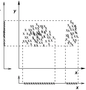
Figure 1: In this example, features x and y are redundant, because feature x provides the same information as feature y with regard to discriminating the two clusters.

y x y x xxxx x xx _x x xx x x x x xx x x x x x x x x x x x x x x x x x

x x x

x x x x x x xx x x x x x x x x xx x x xx xxxxx x x xxx x xxxx

xx xx x x xx x xx x

xxxxxxxxxxxxxx xxxxx x x xx x x x x x x x xx x x x xx_xxx xxx x x x x x x x x

Figure 2: In this example, we consider feature y to be irrelevant, because if we omit x, we have only one cluster, which is uninteresting.

Figure 1 shows an example of feature redundancy for unsupervised learning. Note that the data can be grouped in the same way using only either feature x or feature y. Therefore, we consider features x and y to be redundant. Figure 2 shows an example of an irrelevant feature. Observe that feature y does not contribute to cluster discrimination. Used by itself, feature y leads to a single cluster structure which is uninteresting. Note that irrelevant features can misguide clustering results (especially when there are more irrelevant features than relevant ones). In addition, the situation in unsupervised learning can be more complex than what we depict in Figures 1 and 2. For example, in Figures 3a and b we show the clusters obtained using the feature subsets: {a,b} and {c,d} respectively. Different feature subsets lead to varying cluster structures. Which feature set should we pick?

x

x b

a x x x x x

xx x x x x x xx x x x x x x x x x x x xx x xxxx x x x x x x x x x x

xx _x xx _x

x

x x

x

xxx_x x xx x_{x x} x x xxx xx xx x x x _x x x xxxx

xx xx x x xx x xx_xx x x x x x d c x x x x x x x xx x x x x x x x x x x xx x x x x xx

x x x x x x x x x x x x x x x

x x _x

x x x x x x x x x

x _{x x x}

x x x x x x x x x xx x x xx x x x x xx x x x x x x x xx x xx xxx

x x xx x xxx xx xx x xx x x x x x x x xx x xx x x x x xx x x xx x xx x x x x x x x x x xx x xx x x x x xx xxx x x xx x x x x x x x x x xx x xx x x x x xx x x x xxxx x x x x x x x x x xx x xx x x x x xx

x xxx xxx x xxxxx

(a) (b)

Figure 3: A more complex example. Figure a is the scatterplot of the data on features a and b. Figure b is the scatterplot of the data on features c and d.

The goal of feature selection for unsupervised learning is to find the smallest feature subset that best uncovers “interesting natural” groupings (clusters) from data accord-ing to the chosen criterion.

There may exist multiple redundant feature subset solutions. We are satisfied in finding any one of these solutions. Unlike supervised learning, which has class labels to guide the feature search, in unsupervised learning we need to define what “interesting” and “natural” mean. These are usually represented in the form of criterion functions. We present examples of different criteria in Section 2.3.

Since research in feature selection for unsupervised learning is relatively recent, we hope that this paper will serve as a guide to future researchers. With this aim, we

1. Explore the wrapper framework for unsupervised learning,

2. Identify the issues involved in developing a feature selection algorithm for unsupervised learning within this framework,

3. Suggest ways to tackle these issues,

4. Point out the lessons learned from this endeavor, and 5. Suggest avenues for future research.

Search

Feature

Final

Subset All Features

Criterion Value

Clusters Clusters

Algorithm Clustering

Evaluation Criterion Feature

Feature Subset

Figure 4: Wrapper approach for unsupervised learning.

In particular, this paper investigates the wrapper framework through FSSEM (feature subset se-lection using EM clustering) introduced in (Dy and Brodley, 2000a). Here, the term “EM clustering” refers to the expectation-maximization (EM) algorithm (Dempster et al., 1977; McLachlan and Kr-ishnan, 1997; Moon, 1996; Wolfe, 1970; Wu, 1983) applied to estimating the maximum likelihood parameters of a finite Gaussian mixture. Although we apply the wrapper approach to EM clustering, the framework presented in this paper can be applied to any clustering method. FSSEM serves as an example. We present this paper such that applying a different clustering algorithm or feature selection criteria would only require replacing the corresponding clustering or feature criterion.

In Section 2, we describe FSSEM. In particular, we present the search method, the clustering method, and the two different criteria we selected to guide the feature subset search: scatter separa-bility and maximum likelihood. By exploring the problem in the wrapper framework, we encounter and tackle two issues:

1. different feature subsets have different numbers of clusters, and

2. the feature selection criteria have biases with respect to feature subset dimensionality. In Section 3, we discuss the complications that finding the number of clusters brings to the simulta-neous feature selection/clustering problem and present one solution (FSSEM-k). Section 4 presents a theoretical explanation of why the feature selection criterion biases occur, and Section 5 provides a general normalization scheme which can ameliorate the biases of any feature criterion toward dimension.

Section 6 presents empirical results on both synthetic and real-world data sets designed to an-swer the following questions: (1) Is our feature selection for unsupervised learning algorithm better than clustering on all features? (2) Is using a fixed number of clusters, k, better than using a variable

k in feature search? (3) Does our normalization scheme work? and (4) Which feature selection

criterion is better? Section 7 provides a survey of existing feature selection algorithms. Section 8 provides a summary of the lessons learned from this endeavor. Finally, in Section 9, we suggest avenues for future research.

2. Feature Subset Selection and EM Clustering (FSSEM)

frame-work because we are interested in understanding the interaction between the clustering algorithm and the feature subset search.

Figure 4 illustrates the wrapper approach. Our input is the set of all features. The output is the selected features and the clusters found in this feature subspace. The basic idea is to search through feature subset space, evaluating each candidate subset, Ft, by first clustering in space Ft

using the clustering algorithm and then evaluating the resulting clusters and feature subset using our chosen feature selection criterion. We repeat this process until we find the best feature subset with its corresponding clusters based on our feature evaluation criterion. The wrapper approach divides the task into three components: (1) feature search, (2) clustering algorithm, and (3) feature subset evaluation.

2.1 Feature Search

An exhaustive search of the 2dpossible feature subsets (where d is the number of available features) for the subset that maximizes our selection criterion is computationally intractable. Therefore, a greedy search such as sequential forward or backward elimination (Fukunaga, 1990; Kohavi and John, 1997) is typically used. Sequential searches result in an O(d2) worst case search. In the experiments reported, we applied sequential forward search. Sequential forward search (SFS) starts with zero features and sequentially adds one feature at a time. The feature added is the one that provides the largest criterion value when used in combination with the features chosen. The search stops when adding more features does not improve our chosen feature criterion. SFS is not the best search method, nor does it guarantee an optimal solution. However, SFS is popular because it is simple, fast and provides a reasonable solution. For the purposes of our investigation in this paper, SFS would suffice. One may wish to explore other search methods for their wrapper approach. For example, Kim et al. (2002) applied evolutionary methods. Kittler (1978), and Russell and Norvig (1995) provide good overviews of different search strategies.

2.2 Clustering Algorithm

2.3 Feature Subset Selection Criteria

In this section, we investigate the feature subset evaluation criteria. Here, we define what “inter-estingness” means. There are two general views on this issue. One is that the criteria defining “interestingness” (feature subset selection criteria) should be the criteria used for clustering. The other is that the two criteria need not be the same. Using the same criteria for both clustering and feature selection provides a consistent theoretical optimization formulation. Using two different criteria, on the other hand, presents a natural way of combining two criteria for checks and bal-ances. Proof on which view is better is outside the scope of this paper and is an interesting topic for future research. In this paper, we look at two feature selection criteria (one similar to our clustering criterion and the other with a different bias).

Recall that our goal is to find the feature subset that best discovers “interesting” groupings from data. To select an optimal feature subset, we need a measure to assess cluster quality. The choice of performance criterion is best made by considering the goals of the domain. In studies of performance criteria a common conclusion is: “Different classifications [clusterings] are right for different purposes, so we cannot say any one classification is best.” – Hartigan, 1985 .

In this paper, we do not attempt to determine the best criterion (one can refer to Milligan (1981) on comparative studies of different clustering criteria). We investigate two well-known measures: scatter separability and maximum likelihood. In this section, we describe each criterion, emphasiz-ing the assumptions made by each.

Scatter Separability Criterion: A property typically desired among groupings is cluster sepa-ration. We investigate the scatter matrices and separability criteria used in discriminant analysis (Fukunaga, 1990) as our feature selection criterion. We choose to explore the scatter separability criterion, because it can be used with any clustering method.1 The criteria used in discriminant anal-ysis assume that the features we are interested in are features that can group the data into clusters that are unimodal and separable.

Sw is the within-class scatter matrix and Sb is the between class scatter matrix, and they are

defined as follows:

Sw = k

∑

j=1

πjE{(X−µj)(X−µj)T|ωj}=

k

∑

j=1

πjΣj, (1)

Sb = k

∑

j=1

πj(µj−Mo)(µj−Mo)T, (2)

Mo = E{X}= k

∑

j=1

πjµj, (3)

where πj is the probability that an instance belongs to clusterωj, X is a d-dimensional random

feature vector representing the data, k the number of clusters, µj is the sample mean vector of

clusterωj, Mois the total sample mean,Σjis the sample covariance matrix of clusterωj, and E{·}

is the expected value operator.

Sw measures how scattered the samples are from their cluster means. Sb measures how

scat-tered the cluster means are from the total mean. We would like the distance between each pair of samples in a particular cluster to be as small as possible and the cluster means to be as far apart as possible with respect to the chosen similarity metric (Euclidean, in our case). Among the many possible separability criteria, we choose the trace(S−_w1Sb)criterion because it is invariant under any

nonsingular linear transformation (Fukunaga, 1990). Transformation invariance means that once m features are chosen, any nonsingular linear transformation on these features does not change the criterion value. This implies that we can apply weights to our m features or apply any nonsingular linear transformation or projection to our features and still obtain the same criterion value. This makes the trace(S−1

w Sb) criterion more robust than other variants. S−w1Sb is Sb normalized by the

average cluster covariance. Hence, the larger the value of trace(S−_w1Sb)is, the larger the normalized

distance between clusters is, which results in better cluster discrimination.

Maximum Likelihood (ML) Criterion: By choosing EM clustering, we assume that each group-ing or cluster is Gaussian. We maximize the likelihood of our data given the parameters and our model. Thus, maximum likelihood (ML) tells us how well our model, here a Gaussian mixture, fits the data. Because our clustering criterion is ML, a natural criterion for feature selection is also ML. In this case, the “interesting” groupings are the “natural” groupings, i.e., groupings that are Gaussian.

3. The Need for Finding the Number of Clusters (FSSEM-k)

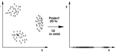
When we are searching for the best subset of features, we run into a new problem: that the number of clusters, k, depends on the feature subset. Figure 5 illustrates this point. In two dimensions (shown on the left) there are three clusters, whereas in one-dimension (shown on the right) there are only two clusters. Using a fixed number of clusters for all feature sets does not model the data in the respective subspace correctly.

x x

xx xxx

x x x x

x xx x x xx xxxxx x x

xxx xxxxx

x xxx x xxx x x x xx x x

x x

x x

x x x

x x x

x x x

x x_x x x x x x xx x

x x xx

x x x x

x xx

xxxxxxxxxxxxxxxxx xxxxxxxxxxxxxx xxxxxxxxxx

Project 2D to

(x-axis) 1D

y y

x x

Figure 5: The number of cluster components varies with dimension.

Unsupervised clustering is made more difficult when we do not know the number of clusters, k. To search for k for a given feature subset, FSSEM-k currently applies Bouman et al.’s method (1998) for merging clusters and adds a Bayesian Information Criterion (BIC) (Schwarz, 1978) penalty term to the log-likelihood criterion. A penalty term is needed because the maximum likelihood estimate increases as more clusters are used. We do not want to end up with the trivial result wherein each data point is considered as an individual cluster. Our new objective function becomes:

F(k,Φ) =log(f(X|Φ))−1

parameters inΦ, and log(f(X|Φ))is the log-likelihood of our observed data X given the parameters

Φ. Note that L andΦvary with k.

Using Bouman et al.’s method (1998), we begin our search for k with a large number of clusters,

Kmax, and then sequentially decrement this number by one until only one cluster remains (a merge

method). Other methods start from k=1 and add more and more clusters as needed (split methods), or perform both split and merge operations (Ueda et al., 1999). To initialize the parameters of the (k−1)th model, two clusters from the kth model are merged. We choose the two clusters among all pairs of clusters in k, which when merged give the minimum difference between F(k−1,Φ) and

F(k,Φ). The parameter values that are not merged retain their value for initialization of the (k−1)th model. The parameters for the merged cluster (l and m) are initialized as follows:

πk−1,(0)

j = πl+πm;

µk_j−1,(0) = πlµl+πmµm

πl+πm ;

Σk−1,(0)

j =

πl(Σl+(µl−µkj−1,(0))(µl−µkj−1,(0))T)+πm(Σm+(µm−µkj−1,(0))(µm−µkj−1,(0))T)

πl+πm ;

where the superscript k−1 indicates the k−1 cluster model and the superscript(0)indicates the first iteration in this reduced order model. For each candidate k, we iterate EM until the change in F(k,Φ)is less thanε(default 0.0001) or up to n (default 500) iterations. Our algorithm outputs the number of clusters k, the parameters, and the clustering assignments that maximize the F(k,Φ)

criterion (our modified ML criterion).

There are myriad ways to find the “optimal” number of clusters k with EM clustering. These methods can be generally grouped into three categories: hypothesis testing methods (McLachlan and Basford, 1988), penalty methods like AIC (Akaike, 1974), BIC (Schwarz, 1978) and MDL (Rissanen, 1983), and Bayesian methods like AutoClass (Cheeseman and Stutz, 1996). Smyth (1996) introduced a new method called Monte Carlo cross-validation (MCCV). For each possible

k value, the average cross-validated likelihood on M runs is computed. Then, the k value with the

highest cross-validated likelihood is selected. In an experimental evaluation, Smyth showed that MCCV and AutoClass found k values that were closer to the number of classes than the k values found with BIC for their data sets. We chose Bouman et al.’s method with BIC, because MCCV is more computationally expensive. MCCV has complexity O(MK_max2 d2NE), where M is the number of cross-validation runs, Kmax is the maximum number of clusters considered, d is the number of

features, N is the number of samples and E is the average number of EM iterations. The complexity of Bouman et al.’s approach is O(K_max2 d2NE0). Furthermore, for k<Kmax, we do not need to

re-initialize EM (because we merged two clusters from k+1) resulting in E0<E. Note that in FSSEM,

we run EM for each candidate feature subset. Thus, in feature selection, the total complexity is the complexity of each complete EM run times the feature search space. Recently, Figueiredo and Jain (2002) presented an efficient algorithm which integrates estimation and model selection for finding the number of clusters using minimum message length (a penalty method). It would be of interest for future work to examine these other ways for finding k coupled with feature selection.

4. Bias of Criterion Values to Dimension

dif-ferent cardinality (corresponding to difdif-ferent dimensionality). In Section 5, we present a solution to this problem.

4.1 Bias of the Scatter Separability Criterion

The separability criterion prefers higher dimensionality; i.e., the criterion value monotonically in-creases as features are added assuming identical clustering assignments (Fukunaga, 1990; Narendra and Fukunaga, 1977). However, the separability criterion may not be monotonically increasing with respect to dimension when the clustering assignments change.

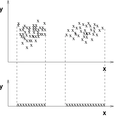
Scatter separability or the trace criterion prefers higher dimensions, intuitively, because data is more scattered in higher dimensions, and mathematically, because more features mean adding more terms in the trace function. Observe that in Figure 6, feature y does not provide additional discrimination to the two-cluster data set. Yet, the trace criterion prefers feature subset{x,y}over feature subset{x}. Ideally, we would like the criterion value to remain the same if the discrimination information is the same.

x x x x x xx_xxxx

xxx

x x

xx

x x x x x _x

x x x x

x xx

x xxxx

x x xxxxxx x

x x x x x x

x x x

x x x

x x x xx

x xx xxx xx x xx xx xx x x x xx

x x

y

x

y

x

xxxxxxxxxxx xxxxxxxxxxxxxxx

Figure 6: An illustration of scatter separability’s bias with dimension.

The following simple example provides us with an intuitive understanding of this bias. Assume that feature subset S1and feature subset S2produce identical clustering assignments, S1⊂S2where

S1 and S2 have d and d+1 features respectively. Assume also that the features are uncorrelated within each cluster. Let Swd and Sbd be the within-class scatter and between-class scatter in dimen-sion d respectively. To compute trace(S−_wd1₊₁Sbd+1) for d+1 dimensions, we simply add a positive

term to the trace(S−_wd1Sbd) value for d dimensions. Swd+1 and Sbd+1 in the d+1 dimensional space

are computed as

Swd+1 =

Swd 0 0 σ2_wd+1

and

Sbd+1 =

Sbd 0 0 σ2_b

d+1

Since

S−_wd1₊₁ =

"

S−_wd1 0 0 _σ21

wd+1

# ,

trace(S−_wd1₊₁Sbd+1)would be trace(S

−1

wdSbd) +

σ2

bd+1

σ2

wd+1

. Sinceσ2_b

d+1 ≥0 andσ

2

wd+1 >0, the trace of the

d+1 clustering will always be greater than or equal to trace of the d clustering under the stated assumptions.

The separability criterion monotonically increases with dimension even when the features are correlated as long as the clustering assignments remain the same. Narendra and Fukunaga (1977) proved that a criterion of the form X_dTS_d−1Xd, where Xdis a d-column vector and Sdis a d×d positive

definite matrix, monotonically increases with dimension. They showed that

X_dT₋₁S−_d−1₁Xd−1=XdTSd−1Xd−

1

b[(C T_{: b)X}

d]2, (4)

where

Xd=

Xd−1

xd

,

S_d−1=

A C

CT _b

,

Xd−1 and C are d−1 column vectors, xd and b are scalars, A is a (d−1)×(d−1) matrix, and

the symbol : means matrix augmentation. We can show that trace(S_w−_d1Sbd) can be expressed as a criterion of the form∑k_j=1XT_jdS_d−1Xjd. Sbd can be expressed as∑

k

j=1ZjbdZ

T

jbd where Zjbd is a d-column vector:

trace(S_w−_d1Sbd) = trace(S

−1

wd

k

∑

j=1

ZjbdZ

T jbd)

= trace(

k

∑

j=1

S−_wd1ZjbdZ

T jbd)

=

k

∑

j=1

trace(S−_wd1ZjbdZ

T jbd)

=

k

∑

j=1

trace(ZT_jbdS−_wd1Zjbd),

since trace(Ap×qBq×p) =trace(Bq×pAp×q)for any rectangular matrices Ap×qand Bq×p.

Because ZT_jb dS

−1

wdZjbd is scalar,

k

∑

j=1

trace(ZT_jbdS−_wd1Zjbd) =

k

∑

j=1

ZT_jbdS−_wd1Zjbd.

4.2 Bias of the Maximum Likelihood (ML) Criterion

Contrary to finding the number of clusters problem, wherein ML increases as the number of model parameters (k) is increased, in feature subset selection, ML prefers lower dimensions. In finding the number of clusters, we try to fit the best Gaussian mixture to the data. The data is fixed and we try to fit our model as best as we can. In feature selection, given different feature spaces, we select the feature subset that is best modeled by a Gaussian mixture.

This bias problem occurs because we define likelihood as the likelihood of the data correspond-ing to the candidate feature subset (see Equation 10 in Appendix B). To avoid this bias, the com-parison can be between two complete (relevant and irrelevant features included) models of the data. In this case, likelihood is defined such that the candidate relevant features are modeled as depen-dent on the clusters, and the irrelevant features are modeled as having no dependence on the cluster variable. The problem with this approach is the need to define a model for the irrelevant features. Vaithyanathan and Dom uses this for document clustering (Vaithyanathan and Dom, 1999). The multinomial distribution for the relevant and irrelevant features is an appropriate model for text fea-tures in document clustering. In other domains, defining models for the irrelevant feafea-tures may be difficult. Moreover, modeling irrelevant features means more parameters to predict. This implies that we still work with all the features, and as we mentioned earlier, algorithms may break down with high dimensions; we may not have enough data to predict all model parameters. One may avoid this problem by adding the assumption of independence among irrelevant features which may not be true. A poorly-fitting irrelevant feature distribution may cause the algorithm to select too many features. Throughout this paper, we use the maximum likelihood definition only for the relevant features.

For a fixed number of samples, ML prefers lower dimensions. The problem occurs when we compare feature set A with feature set B wherein set A is a subset of set B, and the joint probability of a single point(x,y)is less than or equal to its marginal probability(x). For sequential searches, this can lead to the trivial result of selecting only a single feature.

ML prefers lower dimensions for discrete random features. The joint probability mass function of discrete random vectors X and Y is p(X,Y) =p(Y|X)p(X). Since 0≤p(Y|X)≤1, p(X,Y) =

p(Y|X)p(X)≤p(X). Thus, p(X)is always greater than or equal to p(X,Y)for any X . When we deal with continuous random variables, as in this paper, the definition, f(X,Y) = f(Y|X)f(X)still holds, where f(·)is now the probability density function. f(Y|X)is always greater than or equal to zero. However, f(Y|X)can be greater than one. The marginal density f(X)is greater than or equal to the joint probability f(X,Y)iff f(Y|X)≤1.

Theorem 4.1 For a finite multivariate Gaussian mixture, assuming identical clustering assignments

for feature subsets A and B with dimensions dB≥dA, ML(ΦA)≥ML(ΦB)iff

k

∏

j=1

|ΣB|j

|ΣA|j

πj

≥ 1

(2πe)(dB−dA),

whereΦArepresents the parameters andΣAj is the covariance matrix modelling cluster j in feature

Corollary 4.1 For a finite multivariate Gaussian mixture, assuming identical clustering

assign-ments for feature subsets X and(X,Y), where X and Y are disjoint, ML(ΦX)≥ML(ΦXY)iff k

∏

j=1

|ΣYY−ΣY XΣX X−1ΣXY|πjj ≥

1

(2πe)dY,

where the covariance matrix in feature subset(X,Y)is

Σ

X X ΣXY

ΣY X ΣYY

, and dY is the dimension in Y .

We prove Theorem 4.1 and Corollary 4.1 in Appendix B. Theorem 4.1 and Corollary 4.1 reveal the dependencies of comparing the ML criterion for different dimensions. Note that each jth com-ponent of the left hand side term of Corollary 4.1 is the determinant of the conditional covariance of f(Y|X). This covariance term is the covariance of Y eliminating the effects of the conditioning variable X , i.e., the conditional covariance does not depend on X . The right hand side is approx-imately equal to(0.06)dY_{. This means that the ML criterion increases when the feature or feature} subset to be added (Y ) has a generalized variance (determinant of the covariance matrix) smaller than(0.06)dY_{. Ideally, we would like our criterion measure to remain the same when the subsets} re-veal the same clusters. Even when the feature subsets rere-veal the same cluster, Corollary 4.1 informs us that ML decreases or increases depending on whether or not the generalized variance of the new features is greater than or less than a constant respectively.

5. Normalizing the Criterion Values: Cross-Projection Method

The arguments from the previous section illustrate that to apply the ML and trace criteria to feature selection, we need to normalize their values with respect to dimension. A typical approach to normalization is to divide by a penalty factor. For example, for the scatter criterion, we could divide by the dimension, d. Similarly for the ML criterion, we could divide by _(2π1_e)d. But,

1

(2πe)d would not remove the covariance terms due to the increase in dimension. We could also divide log ML by

d, or divide only the portions of the criterion affected by d. The problem with dividing by a penalty

is that it requires specification of a different magic function for each criterion.

The approach we take is to project our clusters to the subspaces that we are comparing. Given two feature subsets, S1and S2, of different dimension, clustering our data using subset S1produces cluster C1. In the same way, we obtain the clustering C2 using the features in subset S2. Which feature subset, S1 or S2, enables us to discover better clusters? Let CRIT(Si,Cj) be the feature

selection criterion value using feature subset Sito represent the data and Cjas the clustering

assign-ment. CRIT(·)represents either of the criteria presented in Section 2.3. We normalize the criterion value for S1, C1as

normalizedValue(S1,C1) =CRIT(S1,C1)·CRIT(S2,C1), and, the criterion value for S2, C2as

normalizedValue(S2,C2) =CRIT(S2,C2)·CRIT(S1,C2).

If normalizedValue(Si,Ci)>normalizedValue(Sj,Cj), we choose feature subset Si. When the

choice of a product or sum operation is arbitrary. Taking the product will be similar to obtaining the geometric mean, and a sum with an arithmetic mean. In general, one should perform normalization based on the semantics of the criterion function. For example, geometric mean would be appropriate for likelihood functions, and an arithmetic mean for the log-likelihood.

When the clustering assignments resulting from different feature subsets, S1and S2, are identical (i.e., C1=C2), the normalizedValue(S1,C1)would be equal to the normalizedValue(S2,C2), which is what we want. More formally:

Proposition 1 Given that C1=C2, equal clustering assignments, for two different feature subsets,

S1and S2, then normalizedValue(S1,C1) =normalizedValue(S2,C2). Proof: From the definition of normalizedValue(·)we have

normalizedValue(S1,C1) = CRIT(S1,C1)·CRIT(S2,C1). Substituting C1=C2,

normalizedValue(S1,C1) = CRIT(S1,C2)·CRIT(S2,C2).

= normalizedValue(S2,C2).

To understand why cross-projection normalization removes some of the bias introduced by the difference in dimension, we focus on normalizedValue(S1,C1). The common factor is C1 (the clusters found using feature subset S1). We measure the criterion values on both feature subsets to evaluate the clusters C1. Since the clusters are projected on both feature subsets, the bias due to data representation and dimension is diminished. The normalized value focuses on the quality of the clusters obtained.

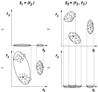
For example, in Figure 7, we would like to see whether subset S1leads to better clusters than subset S2. CRIT(S1,C1) and CRIT(S2,C2) give the criterion values of S1 and S2 for the clusters found in those feature subspaces (see Figures 7a and 7b). We project clustering C1 to S2 in Fig-ure 7c and apply the criterion to obtain CRIT(S2,C1). Similarly, we project C2 to feature space S1 to obtain the result shown in Figure 7d. We measure the result as CRIT(S1,C2). For example, if

ML(S1,C1) is the maximum likelihood of the clusters found in subset S1 (using Equation 10, Ap-pendix B),2 then to compute ML(S2,C1), we use the same cluster assignments, C1, i.e., the E[zi j]’s

(the membership probabilities) for each data point xi remain the same. To compute ML(S2,C1), we apply the maximization-step EM clustering update equations (Equations 7-9 in Appendix A to compute the model parameters in the increased feature space, S2={F2,F3}.

Since we project data in both subsets, we are essentially comparing criteria in the same number of dimensions. We are comparing CRIT(S1,C1) (Figure 7a) with CRIT(S1,C2) (Figure 7d) and

CRIT(S2,C1)(Figure 7c) with CRIT(S2,C2)(Figure 7b). In this example, normalized trace chooses subset S2, because there exists a better cluster separation in both subspaces using C2rather than C1. Normalized ML also chooses subset S2. C2 has a better Gaussian mixture fit (smaller variance clusters) in both subspaces (Figures 7b and d) than C1(Figures 7a and c). Note that the underlying

(a) (b)

(c) (d)

2 2

2 2 F x 3 F F x x x x x x x x

xxxxxxxxxxxxxx xxxxx

x

xxxxxxxxxxxxxx xxxxx

F₃ F₃ x xx xx x x x xx x x xx xxxxx x x xxx x

2 2 3

S = {F } S = {F , F }

x x x x x xx x x x

xx xx

x xx x x F F x x xx x x xx

x xxx x xxx x x x xx x x x x x x x x x x xx x x x xx xx_x xx x x x xx x x xx xxxxx x x xxx x F₃

xxxxx x xxx x xxx

x x x xx x x x x x x x x x

x x_x x x x x x xx x x x xx x x x x x xx

Figure 7: Illustration on normalizing the criterion values. To compare subsets, S1and S2, we project the clustering results of S1, we call C1in (a), to feature space S2as shown in (c). We also project the clustering results of S2, C2 in (b), onto feature space S1 as shown in (d). In (a), tr(S1,C1) =6.094, ML(S1,C1) =1.9×10−64, and log ML(S1,C1) =−146.7. In (b), tr(S2,C2) =9.390, ML(S2,C2) =4.5×10−122, and log ML(S1,C2) =−279.4. In (c), tr(S2,C1) =6.853, ML(S2,C1) =3.6×10−147, and log ML(S2,C1) =−337.2. In (d), tr(S1,C2) =7.358, ML(S1,C2) =2.1×10−64, and log ML(S1,C2) =−146.6. We evaluate subset S1 with normalized tr(S1,C1) =41.76 and subset S2 with normalized

tr(S2,C2) =69.09. In the same way, using ML, the normalized values are: 6.9×10−211 for subset S1 and 9.4×10−186 for subset S2. With log ML, the normalized values are: −483.9 and−426.0 for subsets S1and S2respectively.

assumption behind this normalization scheme is that the clusters found in the new feature space should be consistent with the structure of the data in the previous feature subset. For the ML criterion, this means that Ci should model S1 and S2well. For the trace criterion, this means that

6. Experimental Evaluation

In our experiments, we 1) investigate whether feature selection leads to better clusters than using all the features, 2) examine the results of feature selection with and without criterion normalization, 3) check whether or not finding the number of clusters helps feature selection, and 4) compare the ML and the trace criteria. We first present experiments with synthetic data and then a detailed analysis of the FSSEM variants using four real-world data sets. In this section, we first describe our synthetic Gaussian data, our evaluation methods for the synthetic data, and our EM clustering implementation details. We then present the results of our experiments on the synthetic data. Finally, in Section 6.5, we present and discuss experiments with three benchmark machine learning data sets and one new real world data set.

6.1 Synthetic Gaussian Mixture Data

−4 −3 −2 −1 0 1 2 3

−4 −3 −2 −1 0 1 2 3 4 5 6

feature 1

feature 2

2−class problem

−2 −1 0 1 2 3 4

−4 −3 −2 −1 0 1 2 3 4

feature 1

feature 2

3−class problem

(a) (b)

−4 −2 0 2 4 6 8

−4 −2 0 2 4 6 8

feature 1

feature 2

4−class problem

−8 −6 −4 −2 0 2 4 6 8

−6 −4 −2 0 2 4 6

feature 1

feature 18

5−class problem

−4 −2 0 2 4 6 8

−10 −5 0 5

feature 1

feature 2

5−class and 15 relevant features problem

(c) (d) (e)

Figure 8: Synthetic Gaussian data.

To understand the performance of our algorithm, we experiment with five sets of synthetic Gaus-sian mixture data. For each data set we have “relevant” and “irrelevant” features, where relevant means that we created our k component mixture model using these features. Irrelevant features are generated as Gaussian normal random variables. For all five synthetic data sets, we generated

2-class, 2 relevant features and 3 noise features: The first data set (shown in Figure 8a) consists of two Gaussian clusters, both with covariance matrix, Σ1=Σ2=I and means µ1= (0,0) and µ2 = (0,3). This is similar to the two-class data set used by (Smyth, 1996). There is considerable overlap between the two clusters, and the three additional “noise” features increase the difficulty of the problem.

3-class, 2 relevant features and 3 noise features: The second data set consists of three Gaussian clusters and is shown in Figure 8b. Two clusters have means at (0,0) but the covariance matrices are orthogonal to each other. The third cluster overlaps the tails on the right side of the other two clusters. We add three irrelevant features to the three-class data set used by (Smyth, 1996).

4-class, 2 relevant features and 3 noise features: The third data set (Figure 8c) has four clusters with means at(0,0),(1,4),(5,5)and(5,0)and covariances equal to I. We add three Gaussian normal random “noise” features.

5-class, 5 relevant features and 15 noise features: For the fourth data set, there are twenty fea-tures, but only five are relevant (features{1, 10, 18, 19, 20}). The true means µ were sampled from a uniform distribution on[−5,5]. The elements of the diagonal covariance matricesσ were sampled from a uniform distribution on[0.7,1.5](Fayyad et al., 1998). Figure 8d shows the scatter plot of the data in two of its relevant features.

5-class, 15 relevant features and 5 noise features: The fifth data set (Figure 8e shown in two of its relevant features) has twenty features with fifteen relevant features{1, 2, 3, 5, 8, 9, 10, 11, 12, 13, 14, 16, 17, 18, 20}. The true means µ were sampled from a uniform distribution on

[−5,5]. The elements of the diagonal covariance matricesσwere sampled from a uniform distribution on[0.7,1.5](Fayyad et al., 1998).

6.2 Evaluation Measures

We would like to measure our algorithm’s ability to select relevant features, to correctly identify k, and to find structure in the data (clusters). There are no standard measures for evaluating clusters in the clustering literature (Jain and Dubes, 1988). Moreover, no single clustering assignment (or class label) explains every application (Hartigan, 1985). Nevertheless, we need some measure of perfor-mance. Fisher (1996) provides and discusses different internal and external criteria for measuring clustering performance.

Since we generated the synthetic data, we know the ‘true’ cluster to which each instance be-longs. This ‘true’ cluster is the component that generates that instance. We refer to these ‘true’ clusters as our known ‘class’ labels. Although we used the class labels to measure the performance of FSSEM, we did not use this information during training (i.e., in selecting features and discovering clusters).

different number of clusters using training error. Class error based on training decreases with an increase in the number of clusters, k, with the trivial result of 0% error when each data point is a cluster. To ameliorate this problem, we use ten-fold cross-validation error. Ten-fold cross-validation randomly partitions the data set into ten mutually exclusive subsets. We consider each partition (or fold) as the test set and the rest as the training set. We perform feature selection and clustering on the training set, and compute class error on the test set. For each FSSEM variant, the reported error is the average and standard deviation values from the ten-fold cross-validation runs.

Bayes Error: Since we know the true probability distributions for the synthetic data, we provide the Bayes error (Duda et al., 2001) values to give us the lowest average class error rate achiev-able for these data sets. Instead of a full integration of the error in possibly discontinuous decision regions in multivariate space, we compute the Bayes error experimentally. Using the relevant features and their true distributions, we classify the generated data with an optimal Bayes classifier and calculate the error.

To evaluate the algorithm’s ability to select “relevant” features, we report the average number of features selected, and the average feature recall and precision. Recall and precision are concepts from text retrieval (Salton and McGill, 1983) and are defined here as:

Recall: the number of relevant features in the selected subset divided by the total number of relevant features.

Precision: the number of relevant features in the selected subset divided by the total number of features selected.

These measures give us an indication of the quality of the features selected. High values of preci-sion and recall are desired. Feature precipreci-sion also serves as a measure of how well our dimenpreci-sion normalization scheme (a.k.a. our stopping criterion) works. Finally, to evaluate the clustering al-gorithm’s ability to find the “correct” number of clusters, we report the average number of clusters found.

6.3 Initializing EM and Other Implementation Details

In the EM algorithm, we start with an initial estimate of our parameters,Φ(0), and then iterate using the update equations until convergence. Note that EM is initialized for each new feature subset.

The EM algorithm can get stuck at a local maximum, hence the initialization values are impor-tant. We used the sub-sampling initialization algorithm proposed by Fayyad et al. (1998) with 10% sub-sampling and J=10 sub-sampling iterations. Each sub-sample, Si (i=1, . . . ,J), is randomly

initialized. We run k-means (Duda et al., 2001) on these sub-samples not permitting empty clusters (i.e., when an empty cluster exists at the end of k-means, we reset the empty cluster’s mean equal to the data furthest from its cluster centroid, and re-run k-means). Each sub-sample results in a set of cluster centroids CMi, i, . . . ,J. We then cluster the combined set, CM, of all CMi’s using k-means

initialized by CMiresulting in new centroids FMi. We select the FMi, i=1, . . . ,J, that maximizes

the likelihood of CM as our initial clusters.

the number of iterations because EM converges very slowly near a maximum. We avoid problems with handling singular matrices by adding a scalar (δ=0.000001σ2_{, whereσ}2_{is the average of the} variances of the unclustered data) multiplied to the identity matrix (δI) to each of the component

covariance matricesΣj. This makes the final matrix positive definite (i.e., all eigenvalues are greater

than zero) and hence nonsingular. We constrain our solution away from spurious clusters by deleting clusters with any diagonal element equal to or less thanδ.

6.4 Experiments on Gaussian Mixture Data

We investigate the biases and compare the performance of the different feature selection criteria. We refer to FSSEM using the separability criterion as FSSEM-TR and using ML as FSSEM-ML. Aside from evaluating the performance of these algorithms, we also report the performance of EM (clustering using all the features) to see whether or not feature selection helped in finding more “interesting” structures (i.e., structures that reveal class labels). FSSEM and EM assume a fixed number of clusters, k, equal to the number of classes. We refer to EM clustering and FSSEM with finding the number of clusters as EM-k and FSSEM-k respectively. Due to clarity purposes and space constraints, we only present the relevant tables here. We report the results for all of the evaluation measures presented in Section 6.2 in (Dy and Brodley, 2003).

6.4.1 ML VERSUSTRACE

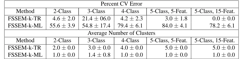
We compare the performance of the different feature selection criteria (k-TR and FSSEM-k-ML) on our synthetic data. We use FSSEM-k rather than FSSEM, because Section 6.4.3 shows that feature selection with finding k (FSSEM-k) is better than feature selection with fixed k (FSSEM). Table 1 shows the cross-validated (CV) error and average number of clusters results for trace and ML on the five data sets.

Percent CV Error

Method 2-Class 3-Class 4-Class 5-Class, 5-Feat. 5-Class, 15-Feat. FSSEM-k-TR 4.6±2.0 21.4±06.0 4.2±2.3 3.0±1.8 0.0±0.0 FSSEM-k-ML 55.6±3.9 54.8±17.4 79.4±6.1 84.0±4.1 78.2±6.1

Average Number of Clusters

Method 2-Class 3-Class 4-Class 5-Class, 5-Feat. 5-Class, 15-Feat. FSSEM-k-TR 2.0±0.0 3.0±0.0 4.0±0.0 5.0±0.0 5.0±0.0 FSSEM-k-ML 1.0±0.0 1.4±0.8 1.0±0.0 1.0±0.0 1.0±0.0

Table 1: Cross-validated error and average number of clusters for TR versus FSSEM-k-ML applied to the simulated Gaussian mixture data.

6.4.2 RAWDATAVERSUSSTANDARDIZEDDATA

In the previous subsection, ML performed worse than trace for our synthetic data, because ML prefers features with low variance and fewer clusters (our noise features have lower variance than the relevant features). In this subsection, we investigate whether standardizing the data in each dimension (i.e., normalizing each dimension to yield a variance equal to one) would eliminate this bias. Standardizing data is sometimes done as a pre-processing step in data analysis algorithms to equalize the weight contributed by each feature. We would also like to know how standardization affects the performance of the other FSSEM variants.

Let X be a random data vector and Xf ( f =1. . .d) be the elements of the vector, where d is

the number of features. We standardize X by dividing each element by the corresponding feature standard deviation (Xf/σf, whereσf is the standard deviation for feature f ).

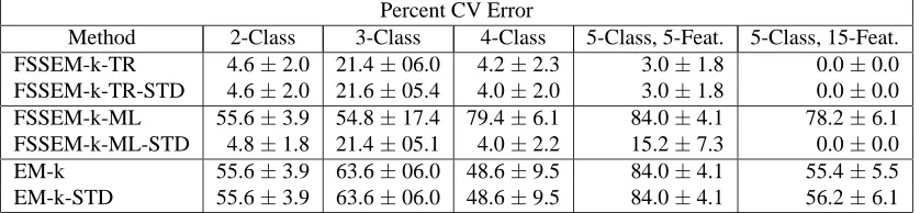
Table 2 reports the CV error. Additional experimental results can be found in (Dy and Brodley, 2003). Aside from the FSSEM variants, we examine the effect of standardizing data on EM-k, clustering with finding the number of clusters using all the features. We represent the corresponding variant on standardized data with the suffix “-STD”. The results show that only FSSEM-k-ML is affected by standardizing data. The trace criterion computes the between-class scatter normalized by the average within-class scatter and is invariant to any linear transformation. Since standardizing data is a linear transformation, the trace criterion results remain unchanged.

Standardizing data improves ML’s performance. It eliminates ML’s bias to lower overall vari-ance features. Assuming equal varivari-ance clusters, ML prefers a single Gaussian cluster over two well-separated Gaussian clusters. But, after standardization, the two Gaussian clusters become more favorable because each of the two clusters now has lower variance (i.e., higher probabilities) than the single cluster noise feature. Observe that when we now compare FSSEM-k-TR-STD or FSSEM-k-TR with FSSEM-k-ML-STD, the performance is similar for all our data sets. These results show that scale invariance is an important property for a feature evaluation criterion. If a criterion is not scale invariant such as ML, in this case, pre-processing by standardizing the data in each dimension is necessary. Scale invariance can be incorporated to the ML criterion by mod-ifying the function as presented in (Dy and Brodley, 2003). Throughout the rest of the paper, we standardize the data before feature selection and clustering.

Percent CV Error

Method 2-Class 3-Class 4-Class 5-Class, 5-Feat. 5-Class, 15-Feat. FSSEM-k-TR 4.6±2.0 21.4±06.0 4.2±2.3 3.0±1.8 0.0±0.0 FSSEM-k-TR-STD 4.6±2.0 21.6±05.4 4.0±2.0 3.0±1.8 0.0±0.0 FSSEM-k-ML 55.6±3.9 54.8±17.4 79.4±6.1 84.0±4.1 78.2±6.1 FSSEM-k-ML-STD 4.8±1.8 21.4±05.1 4.0±2.2 15.2±7.3 0.0±0.0

EM-k 55.6±3.9 63.6±06.0 48.6±9.5 84.0±4.1 55.4±5.5

EM-k-STD 55.6±3.9 63.6±06.0 48.6±9.5 84.0±4.1 56.2±6.1

Table 2: Percent CV error of FSSEM variants on standardized and raw data.

6.4.3 FEATURESEARCH WITHFIXEDk VERSUSSEARCH FORk

of clusters, k, in our approach. In this section, we investigate whether finding k yields better per-formance than using a fixed number of clusters. We represent the FSSEM and EM variants using a fixed number of clusters (equal to the known classes) as FSSEM and EM. FSSEM-k and EM-k stand for FSSEM and EM with searching for k. Tables 3 and 4 summarize the CV error, average number of cluster, feature precision and recall results of the different algorithms on our five synthetic data sets.

Percent CV Error

Method 2-Class 3-Class 4-Class 5-Class, 5-Feat. 5-Class, 15-Feat. FSSEM-TR-STD 4.4±02.0 37.6±05.6 7.4±11.0 21.2±20.7 14.4±22.2 FSSEM-k-TR-STD 4.6±02.0 21.6±05.4 4.0±02.0 3.0±01.8 0.0±00.0 FSSEM-ML-STD 7.8±05.5 22.8±06.6 3.6±01.7 15.4±09.5 4.8±07.5 FSSEM-k-ML-STD 4.8±01.8 21.4±05.1 4.0±02.2 15.2±07.3 0.0±00.0 EM-STD 22.4±15.1 30.8±13.1 23.2±10.1 48.2±07.5 10.2±11.0 EM-k-STD 55.6±03.9 63.6±06.0 48.6±09.5 84.0±04.1 56.2±06.1

Bayes 5.4±00.0 20.4±00.0 3.4±00.0 0.8±00.0 0.0±00.0

Average Number of Clusters

Method 2-Class 3-Class 4-Class 5-Class, 5-Feat. 5-Class, 15-Feat. FSSEM-TR-STD fixed at 2 fixed at 3 fixed at 4 fixed at 5 fixed at 5 FSSEM-k-TR-STD 2.0±0.0 3.0±0.0 4.0±0.0 5.0±0.0 5.0±0.0 FSSEM-ML-STD fixed at 2 fixed at 3 fixed at 4 fixed at 5 fixed at 5 FSSEM-k-ML-STD 2.0±0.0 3.0±0.0 4.0±0.0 4.2±0.4 5.0±0.0

EM-STD fixed at 2 fixed at 3 fixed at 4 fixed at 5 fixed at 5

EM-k-STD 1.0±0.0 1.0±0.0 2.0±0.0 1.0±0.0 2.1±0.3

Table 3: Percent CV error and average number of cluster results on FSSEM and EM with fixed number of clusters versus finding the number of clusters.

Looking first at FSSEM-k-TR-STD compared to FSSEM-TR-STD, we see that including order identification (FSSEM-k-TR-STD) with feature selection results in lower CV error for the trace criterion. For all data sets except the two-class data, FSSEM-k-TR-STD had significantly lower CV error than FSSEM-TR-STD. Adding the search for k within the feature subset selection search allows the algorithm to find the relevant features (an average of 0.796 feature recall for FSSEM-k-TR-STD versus 0.656 for FSSEM-FSSEM-k-TR-STD).3_{This is because the best number of clusters depends} on the chosen feature subset. For example, on closer examination, we noted that on the three-class problem when k is fixed at three, the clusters formed by feature 1 are better separated than clusters that are formed by features 1 and 2 together. As a consequence, FSSEM-TR-STD did not select feature 2. When k is made variable during the feature search, FSSEM-k-TR-STD finds two clusters in feature 1. When feature 2 is considered with feature 1, three or more clusters are found resulting in higher separability.

In the same way, FSSEM-k-ML-STD was better than fixing k, FSSEM-ML-STD, for all data sets in terms of CV error except for the four-class data. FSSEM-k-ML-STD performed slightly better than FSSEM-ML-STD for all the data sets in terms of feature precision and recall. This

Average Feature Precision

Method 2-Class 3-Class 4-Class 5-Class, 5-Feat. 5-Class, 15-Feat. FSSEM-TR-STD 0.62±0.26 0.56±0.24 0.68±0.17 0.95±0.15 1.00±0.00 FSSEM-k-TR-STD 0.57±0.23 0.65±0.05 0.53±0.07 1.00±0.00 1.00±0.00 FSSEM-ML-STD 0.24±0.05 0.52±0.17 0.53±0.10 0.98±0.05 1.00±0.00 FSSEM-k-ML-STD 0.33±0.00 0.67±0.13 0.50±0.00 1.00±0.00 1.00±0.00 EM-k 0.20±0.00 0.20±0.00 0.20±0.00 0.25±0.00 0.75±0.00 EM-k-STD 0.20±0.00 0.20±0.00 0.20±0.00 0.25±0.00 0.75±0.00

Average Feature Recall

Method 2-Class 3-Class 4-Class 5-Class, 5-Feat. 5-Class, 15-Feat. FSSEM-TR-STD 1.00±0.00 0.55±0.15 0.95±0.15 0.46±0.20 0.32±0.19 FSSEM-k-TR-STD 1.00±0.00 1.00±0.00 1.00±0.00 0.62±0.06 0.36±0.13 FSSEM-ML-STD 1.00±0.00 1.00±0.00 1.00±0.00 0.74±0.13 0.41±0.20 FSSEM-k-ML-STD 1.00±0.00 1.00±0.00 1.00±0.00 0.72±0.16 0.51±0.14 EM-k 1.00±0.00 1.00±0.00 1.00±0.00 1.00±0.00 1.00±0.00 EM-k-STD 1.00±0.00 1.00±0.00 1.00±0.00 1.00±0.00 1.00±0.00

Table 4: Average feature precision and recall obtained by FSSEM with a fixed number of clusters versus FSSEM with finding the number of clusters.

shows that incorporating finding k helps in selecting the “relevant” features. EM-STD had lower CV error than k-STD due to prior knowledge about the correct number of clusters. Both EM-STD and EM-k-EM-STD had poorer performance than FSSEM-k-TR/ML-EM-STD, because of the retained noisy features.

6.4.4 FEATURECRITERIONNORMALIZATIONVERSUSWITHOUTNORMALIZATION

Percent CV Error

Method 2-Class 3-Class 4-Class 5-Class, 5-Feat. 5-Class, 15-Feat. FSSEM-k-TR-STD-notnorm 4.6±2.0 23.4±6.5 4.2±2.3 2.6±1.3 0.0±0.0

FSSEM-k-TR-STD 4.6±2.0 21.6±5.4 4.0±2.0 3.0±1.8 0.0±0.0

FSSEM-k-ML-STD-notnorm 4.6±2.2 36.2±4.2 48.2±9.4 63.6±4.9 46.8±6.2

FSSEM-k-ML-STD 4.8±1.8 21.4±5.1 4.0±2.2 15.2±7.3 0.0±0.0

Bayes 5.4±0.0 20.4±0.0 3.4±0.0 0.8±0.0 0.0±0.0

Average Number of Features Selected

Method 2-Class 3-Class 4-Class 5-Class, 5-Feat. 5-Class, 15-Feat. FSSEM-k-TR-STD-notnorm 2.30±0.46 3.00±0.00 3.90±0.30 3.30±0.46 9.70±0.46 FSSEM-k-TR-STD 2.00±0.63 3.10±0.30 3.80±0.40 3.10±0.30 5.40±1.96 FSSEM-k-ML-STD-notnorm 1.00±0.00 1.00±0.00 1.00±0.00 1.00±0.00 1.00±0.00 FSSEM-k-ML-STD 3.00±0.00 3.10±0.54 4.00±0.00 3.60±0.80 7.70±2.10

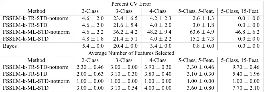
Table 5 presents the CV error and average number of features selected by feature selection with cross-projection criterion normalization versus without (those with suffix “notnorm”). Here and throughout the paper, we refer to normalization as the feature normalization scheme (cross-projection method) described in Section 5. For the trace criterion, without normalization did not affect the CV error. However, normalization achieved similar CV error performance using fewer features than without normalization. For the ML criterion, criterion normalization is definitely needed. Note that without, FSSEM-k-ML-STD-notnorm selected only a single feature for each data set resulting in worse CV error performance than with normalization (except for the two-class data which has only one relevant feature).

6.4.5 FEATURESELECTIONVERSUSWITHOUTFEATURESELECTION

In all cases, feature selection (FSSEM, FSSEM-k) obtained better results than without feature se-lection (EM, EM-k) as reported in Table 3. Note that for our data sets, the noise features misled EM-k-STD, leading to fewer clusters than the “true” k. Observe too that FSSEM-k was able to find approximately the true number of clusters for the different data sets.

In this subsection, we experiment on the sensitivity of the FSSEM variants to the number of noise features. Figures 9a-e plot the cross-validation error, average number of clusters, average number of noise features, feature precision and recall respectively of feature selection (FSSEM-k-TR-STD and FSSEM-k-ML-STD) and without feature selection (EM-k-STD) as more and more noise features are added to the four-class data. Note that the CV error performance, average number of clusters, average number of selected features and feature recall for the feature selection algorithms are more or less constant throughout and are approximately equal to clustering with no noise. The feature precision and recall plots reveal that the CV error performance of feature selection was not affected by noise, because the FSSEM-k variants were able to select the relevant features (recall=1) and discard the noisy features (high precision). Figure 9 demonstrates the need for feature selection as irrelevant features can mislead clustering results (reflected by EM-k-STD’s performance as more and more noise features are added).

6.4.6 CONCLUSIONS ONEXPERIMENTS WITHSYNTHETICDATA

Experiments on simulated Gaussian mixture data reveal that:

• Standardizing the data before feature subset selection in conjunction with the ML criterion is needed to remove ML’s preference for low variance features.

• Order identification led to better results than fixing k, because different feature subsets have different number of clusters as illustrated in Section 3.

• The criterion normalization scheme (cross-projection) introduced in Section 5 removed the biases of trace and ML with respect to dimension. The normalization scheme enabled feature selection with trace to remove “redundant” features and prevented feature selection with ML from selecting only a single feature (a trivial result).

• Both ML and trace with feature selection performed equally well for our five data sets. Both criteria were able to find the “relevant” features.

0 2 4 6 8 10 12 14 16 18 0

10 20 30 40 50 60 70 80

Number of Noise Features

Percent CV−Error

FSSEM−k−TR−STD FSSEM−k−ML−STD EM−k−STD

0 2 4 6 8 10 12 14 16 18 1

1.5 2 2.5 3 3.5 4 4.5

Number of Noise Features

Average Number of Clusters

FSSEM−k−TR−STD FSSEM−k−ML−STD EM−k−STD

(a) (b)

0 2 4 6 8 10 12 14 16 18 2

4 6 8 10 12 14 16 18 20

Number of Noise Features

Average Number of Features

FSSEM−k−TR−STD FSSEM−k−ML−STD EM−k−STD

0 2 4 6 8 10 12 14 16 18 0.1

0.2 0.3 0.4 0.5 0.6 0.7 0.8 0.9 1

Number of Noise Features

Average Feature Precision

FSSEM−k−TR−STD FSSEM−k−ML−STD EM−k−STD

(c) (d)

0 2 4 6 8 10 12 14 16 18 0

0.2 0.4 0.6 0.8 1 1.2 1.4 1.6 1.8 2

Number of Noise Features

Average Feature Recall

FSSEM−k−TR−STD FSSEM−k−ML−STD EM−k−STD

(e)

Figure 9: Feature selection versus without feature selection on the four-class data.

6.5 Experiments on Real Data

image data which we collected from IUPUI medical center (Dy et al., 2003; Dy et al., 1999). Al-though for each data set the class information is known, we remove the class labels during training. Unlike synthetic data, we do not know the “true” number of (Gaussian) clusters for real-world data sets. Each class may be composed of many Gaussian clusters. Moreover, the clusters may not even have a Gaussian distribution. To see whether the clustering algorithms found clusters that correspond to classes (wherein a class can be multi-modal), we compute the cross-validated class error in the same way as for the synthetic Gaussian data. On real data sets, we do not know the “relevant” features. Hence, we cannot compute precision and recall and therefore report only the average number of features selected and the average number of clusters found.

Although we use class error as a measure of cluster performance, we should not let it misguide us in its interpretation. Cluster quality or interestingness is difficult to measure because it depends on the particular application. This is a major distinction between unsupervised clustering and su-pervised learning. Here, class error is just one interpretation of the data. We can also measure cluster performance in terms of the trace criterion and the ML criterion. Naturally, FSSEM-k-TR and FSSEM-TR performed best in terms of trace; and, FSSEM-k-ML and FSSEM-ML were best in terms of maximum likelihood. Choosing either TR or ML depends on your application goals. If you are interested in finding the features that best separate the data, use FSSEM-k-TR. If you are interested in finding features that model Gaussian clusters best, use FSSEM-k-ML.

To illustrate the generality and ease of applying other clustering methods in the wrapper frame-work, we also show the results for different variants of feature selection wrapped around the k-means clustering algorithm (Forgy, 1965; Duda et al., 2001) coupled with the TR and ML criteria. We use sequential forward search for feature search. To find the number of clusters, we apply the BIC penalty criterion (Pelleg and Moore, 2000). We use the following acronyms throughout the rest of the paper: Kmeans stands for the k-means algorithm, FSS-Kmeans stands for feature selection wrapped around k-means, TR represents the trace criterion for feature evaluation, ML represents ML criterion for evaluating features, “-k-” represents that the variant finds the number of clusters, and “-STD” shows that the data was standardized such that each feature has variance equal to one.

Since cluster quality depends on the initialization method used for clustering, we performed EM clustering using three different initialization methods:

1. Initialize using ten k-means starts with each k-means initialized by a random seed, then pick the final clustering corresponding to the highest likelihood.

2. Ten random re-starts.

3. Fayyad et al.’s method as described earlier in Section 6.3 (Fayyad et al., 1998).

Iris Data and FSSEM Variants

Method %CV Error Ave. No. of Clusters Ave. No. of Features

FSSEM-TR-STD-1 2.7±04.4 fixed at 3 3.5±0.7

FSSEM-k-TR-STD-1 4.7±05.2 3.1±0.3 2.7±0.5

FSSEM-ML-STD-1 7.3±12.1 fixed at 3 3.6±0.9

FSSEM-k-ML-STD-1 3.3±04.5 3.0±0.0 2.5±0.5

EM-STD-1 3.3±05.4 fixed at 3 fixed at 4

EM-k-STD-1 42.0±14.3 2.2±0.6 fixed at 4

Iris Data and FSS-Kmeans Variants

Method %CV Error Ave. No. of Clusters Ave. No. of Features

FSS-Kmeans-TR-STD-2 2.7±03.3 fixed at 3 1.9±0.3

FSS-Kmeans-k-TR-STD-2 13.3±09.4 4.5±0.7 2.3±0.5

FSS-Kmeans-ML-STD-2 2.0±03.1 fixed at 3 2.0±0.0

FSS-Kmeans-k-ML-STD-2 4.7±04.3 3.4±0.5 2.4±0.5

Kmeans-STD-2 17.3±10.8 fixed at 3 fixed at 4

Kmeans-k-STD-2 44.0±11.2 2.0±0.0 fixed at 4

Table 6: Results for the different variants on the iris data.

6.5.1 IRISDATA

We first look at the simplest case, the Iris data. This data has three classes, four features, and 150 instances. Fayyad et. al’s method of initialization works best for large data sets. Since the Iris data only has a few number of instances and classes that are well-separated, ten k-means starts provided the consistently best result for initializing EM clustering across the different methods. Table 6 summarizes the results for the different variants of FSSEM compared to EM clustering without feature selection. For the iris data, we set Kmaxin FSSEM-k equal to six, and for FSSEM we fixed k

at three (equal to the number of labeled classes). The CV error for k-TR-STD and FSSEM-k-ML-STD are much better than EM-k-STD. This means that when you do not know the “true” number of clusters, feature selection helps find good clusters. FSSEM-k even found the “correct” number of clusters. EM clustering with the “true” number of clusters (EM-STD) gave good results. Feature selection, in this case, did not improve the CV-error of EM-STD, however, they produced similar error rates with fewer features. FSSEM with the different variants consistently chose feature 3 (petal-length), and feature 4 (petal-width). In fact, we learned from this experiment that only these two features are needed to correctly cluster the iris data to three groups corresponding to iris-setosa, iris-versicolor and iris-viginica. Figures 10 (a) and (b) show the clustering results as a scatterplot on the first two features chosen by FSSEM-k-TR and FSSEM-k-ML respectively. The results for feature selection wrapped around k-means are also shown in Table 6. We can infer similar conclusions from the results on FSS-Kmeans variants as with the FSSEM variants for this data set.

6.5.2 WINEDATA

The wine data has three classes, thirteen features and 178 instances. For this data, we set Kmax

0.5 1 1.5 2 2.5 3 3.5 4 0

0.5 1 1.5 2 2.5 3 3.5

feature 3

feature 4

0.5 1 1.5 2 2.5 3 3.5 4 0

0.5 1 1.5 2 2.5 3 3.5

feature 3

feature 4

(a) (b)

Figure 10: The scatter plots on iris data using the first two features chosen by FSSEM-k-TR (a) and FSSEM-k-ML (b). , × and5 represent the different class assignments. ◦ are the cluster means, and the ellipses are the covariances corresponding to the clusters discovered by FSSEM-k-TR and FSSEM-k-ML.

Wine Data and FSSEM Variants

Method %CV Error Ave. No. of Clusters Ave. No. of Features

FSSEM-TR-STD-1 44.0±08.1 fixed at 3 1.4±0.5

FSSEM-k-TR-STD-1 12.4±13.0 3.6±0.8 3.8±1.8

FSSEM-ML-STD-1 30.6±21.8 fixed at 3 2.9±0.8

FSSEM-k-ML-STD-1 23.6±14.4 3.9±0.8 3.0±0.8

EM-STD-1 10.0±17.3 fixed at 3 fixed at 13

EM-k-STD-1 37.1±12.6 3.2±0.4 fixed at 13

Wine Data and FSS-Kmeans Variants

Method %CV Error Ave. No. of Clusters Ave. No. of Features

FSS-Kmeans-TR-STD-2 37.3±14.0 fixed at 3 1.0±0.0

FSS-Kmeans-k-TR-STD-2 28.1±09.6 3.6±0.5 2.5±0.9

FSS-Kmeans-ML-STD-2 16.1±09.9 fixed at 3 3.1±0.3

FSS-Kmeans-k-ML-STD-2 18.5±07.2 4.2±0.6 3.1±0.7

Kmeans-STD-2 0.0±00.0 fixed at 3 fixed at 13

Kmeans-k-STD-2 33.4±21.3 2.6±0.8 fixed at 13

Table 7: Results for the different variants on the wine data set.

1.5 2 2.5 3 3.5 4 4.5 5 5.5 6 0.5

1 1.5 2 2.5 3 3.5 4 4.5 5 5.5

feature 12

feature 13

0.5 1 1.5 2 2.5 3 3.5 4 4.5 5 5.5 0.5

1 1.5 2 2.5 3 3.5 4 4.5 5 5.5

feature 2

feature 13

(a) (b)

Figure 11: The scatter plots on the wine data using the first two features chosen by FSSEM-k-TR (a) and FSSEM-k-ML (b). ?, × and5 represent the different class assignments. ◦ are the cluster means, and the ellipses are the covariances corresponding to the clusters discovered by FSSEM-k-TR and FSS-Kmeans-k-ML.

FSS-Kmeans-k-ML selected features{2,13,12}.4_{Features 12 and 13 stand for “OD280-OD315 of} diluted wines” and “proline.”

6.5.3 IONOSPHEREDATA

The radar data is collected from a phased array of sixteen high-frequency antennas. The targets are free electrons in the atmosphere. Classes label the data as either good (radar returns showing structure in the ionosphere) or bad returns. There are 351 instances with 34 continuous attributes (measuring time of pulse and pulse number). Features 1 and 2 are discarded, because their values are constant or discrete for all instances. Constant feature values produce an infinite likelihood value for a Gaussian mixture model. Discrete feature values with discrete levels less than or equal to the number of clusters also produce an infinite likelihood value for a finite Gaussian mixture model.

Table 8 reports the ten-fold cross-validation error and the number of clusters found by the differ-ent EM and FSSEM algorithms. For the ionosphere data, we set Kmaxin FSSEM-k equal to ten, and

fixed k at two (equal to the number of labeled classes) in FSSEM. FSSEM-k-ML and EM clustering with “k” known performed better in terms of CV error compared to the rest of the EM variants. Note that FSSEM-k-ML gave comparable performance with EM using fewer features and with no knowledge of the “true” number of clusters. Table 8 also shows the results for the different k-means variants. FSS-Kmeans-k-ML-STD obtains the best CV error followed closely by FSS-Kmeans-ML-STD. Interestingly, these two methods and FSSEM-k-ML all chose features 5 and 3 (based on the original 34 features) as their first two features.

Figures 12a and b present scatterplots of the ionosphere data on the first two features chosen by FSSEM-k-TR and FSSEM-k-ML together with their corresponding means (in◦’s) and covariances (in ellipses) discovered. Observe that FSSEM-k-TR favored the clusters and features in Figure 12a because the clusters are well separated. On the other hand, FSSEM-k-ML favored the clusters in Figure 12b, which have small generalized variances. Since the ML criterion matches the ionosphere