Predicting Genetic Interactions in
Caenorhabditis
elegans
using Machine Learning
by
Patrycja Vasilyev Missiuro
B.S., M.S. Electrical Engineering and Computer Science,
Massachusetts Institute of Technology, 2001
Submitted to the Department of Electrical Engineering and Computer
Science
in partial fulfillment of the requirements for the degree of
Doctor of Philosophy
at the
MASSACHUSETTS INSTITUTE OF TECHNOLOGY
February 2010
Massachusetts Institute of Technology 2010. All rights reserved.
Author . . . .
Department of Electrical Engineering and Computer Science
December 18, 2009
Certified by. . . .
Tommi S. Jaakkola
Professor of Electrical Engineering and Computer Science
Thesis Supervisor
Certified by. . . .
Hui Ge
Research Fellow at the Whitehead Institute
Thesis Supervisor
Accepted by . . . .
Terry P. Orlando
Chairman, Department Committee on Graduate Students
Predicting Genetic Interactions in
Caenorhabditis elegans
using
Machine Learning
by
Patrycja Vasilyev Missiuro
Submitted to the Department of Electrical Engineering and Computer Science on December 18, 2009, in partial fulfillment of the
requirements for the degree of Doctor of Philosophy
Abstract
The presented work develops a set of machine learning and other computational techniques to investigate and predict gene properties across a variety of biological datasets. In particular, our main goal is the discovery of genetic interactions based on sparse and incomplete information. In our development, we use gene data from two model organisms, Caenorhabditis elegans and Saccharomyces cerevisiae.
Our first method,information flow, uses circuit theory to evaluate the importance of a protein in an interactome. We find that proteins with high i-flow scores mediate information exchange between functional modules. We also show that increasing in-formation flow scores strongly correlate with the likelihood of observing lethality or pleiotropy as well as observing genetic interactions. Our metric significantly outper-forms other established network metrics such as degree or betweenness.
Next, we show how Bayesian sets can be applied to gain intuition as to which datasets are the most relevant for predicting genetic interactions. In order to directly apply this method to microarray data, we extend Bayesian sets to handle continuous variables. Using Bayesian sets, we show that genetically interacting genes tend to share phenotypes but are not necessarily co-localized. Additionally, they have similar development and aging temporal expression profiles.
One of the major difficulties in dealing with biological data is the problem of incomplete datasets. We describe a novel application ofcollaborative filtering(CF) in order to predict missing values in the biological datasets. We adapt the factorization-based and the neighborhood-aware CF [13] to deal with a mixture of continuous and discrete entries. We use collaborative filtering to input missing values, assess how much information relevant to genetic interactions is present, and, finally, to predict genetic interactions. We also show how CF can reduce input dimensionality.
Our last development is the application of Support Vector Machines (SVM), an adapted machine learning classification method, to predicting genetic interactions. We find that SVM with nonlinear radial basis function (RBF) kernel has greater predictive power over CF. Its performance, however, greatly benefits from using CF to fill in missing entries in the input data. We show that SVM performance further
improves if we constrain the group of genes to a specific functional category.
Throughout this thesis, we emphasize the features of the studied datasets and explain our findings from a biological perspective. In this respect, we hope that this work possesses an independent biological significance. The final step would be to confirm our predictions experimentally. This would allow us to gain new insights into C. elegans biology: specific genes orchestrating developmental and regulatory pathways, response to stress, etc.
Thesis Supervisor: Tommi S. Jaakkola
Title: Professor of Electrical Engineering and Computer Science Thesis Supervisor: Hui Ge
Acknowledgments
Research is a challenging and time-consuming effort and the final written product is only a small snapshot of the total work done. In my opinion, the greatest benefit of completing this PhD thesis is that it taught me how to think and gave me the mental preparedness for doing future research work. Not that I did not have doubts in the process... I succeeded thanks to the guidance of my academic mentors and the enormous support of my family and friends.
First and foremost, I want to thank my advisors for their support throughout development of this thesis. Doctor Hui Ge is an incredibly insightful thinker and has always kept my focus on the big picture and provided me with biological insight and knowledge which I, as a computer scientist, lack. Professor Tommi Jaakkola has provided me with his invaluable input on the computational methods. He has led me numerous times to very insightful observations and conclusions that I would have never reached alone, and provided suggestions as to possible research directions. Professor Manolis Kellis has always been enthusiastic to give me his feedback; he has been a friend and a mentor throughout my undergraduate and graduate years. Finally, I would like to thank Professor Richard Young, who as a biologist, was looking at my work from a different angle than merely computational.
I want to thank my incredible husband, Dmitry Vasilyev, for his enormous emo-tional support, love, and calmness that kept me going. Had it not been for him, I am convinced I would not be writing this today. Thanks to my mom, dad, siblings: Julia Aurelia, Justynian and Ewaryst, aunts and uncles, for rooting for me. Special thanks to Sasha and Andrew for their words of child wisdom. I want to thank my friends: Ewa, Irina, Jennifer, Julie, Tim, Monika, Kesheng, Brian, Alex, Matt, Brittany, Ben, David, Tom, Alec, Olivier, Nikita and many others who have made me laugh and allowed me to relax and some of whom were willing to travel with me thousands of miles across this beautiful country. While the first four ladies stayed awake while proofreading my thesis, several others stayed awake while hearing my practice talk.
PhD thesis while renovating a multi-family fixer-upper and being a landlord.
I dedicate this thesis to my dear parents - Wies̷lawa and W̷lodzimierz who both made great sacrifices for me and my siblings to come to this country. My father has always encouraged me to learn new things and seek new hobbies as he is still doing today. My mom has shown incredible strength, energy and dedication and has always been my role model.
Contents
1 Introduction 27
1 .1 Motivation & Objectives . . . 27
1 .2 What are genetic interactions? . . . 28
1 .3 Prior research on genetic interactions and biological networks . . . 30
1 .3.1 Hypothesized properties of genetically interacting pairs . . . . 30
1.3.2 Current computational approaches to identify genetic interactions 32 1 .4 Thesis summary . . . 34
2 Biology Background 37 2.1 Caenorhabditis elegansas a model organism . . . 37
2.2 Saccharomyces cerevisiaeas a model organism . . . 42
2.3 High-throughput datasets . . . 43
2.3.1 DNA Microarrays . . . 43
2.3.2 Spatial expression patterns . . . 46
2.3.3 Phenotypes . . . 47
2.3.4 Protein interaction networks . . . 49
2.3.5 microRNAs . . . 50
2.3.6 Kinase families . . . 51
2.3.7 Phosphatase families . . . 52
2.3.8 Known genetic interactions . . . 53
3Information flow method 57
3.1 Motivation . . . 57
3.2 Relevant network algorithms and metrics . . . 60
3.2.1 Degree . . . 60
3.2.2 Betweenness . . . 61
3.3 The information flow model . . . 62
3.3.1 The Iflow algorithm . . . 62
3.3.2 Partition of interactome into modules algorithm . . . 65
3.4 Experimental results and conclusions . . . 66
3.4.1Information flow model considers interaction confidence scores and all possible paths in protein networks . . . 66
3.4.2 Information flow is a strong predictor of essentiality and pleiotropy 69 3.4.3 Proteins of high information flow and low betweenness show a high likelihood for being essential or pleiotropic . . . 71
3.4.4 The ranks of information flow scores are more consistent than betweenness when a large amount of low-confidence data is added 77 3.4.5 Information flow analysis of a muscle interactome network re-veals genes important for muscle function in C. elegans . . . . 79
3.4.6 Information flow discovers crucial proteins in signaling networks 83 3.5 Materials . . . 85
3.5.1 Data sources . . . 85
3.5.2 RNA interference . . . 86
3.6 Discussion . . . 86
4 Finding groupings among genes with Bayesian Sets 91 4.1 Introduction to Bayesian sets . . . 92
4.1 .1 Method description . . . 93
4.1 .2 Binary data model . . . 95
4.1.3 Using binary Bayesian sets to group genes based on their local-ization and phenotypes . . . 96
4.2 Extensions to Bayesian sets for continuous data . . . 1 01 4.2.1 Bayesian sets model for continuous data - variant 1. . . 101 4.2.2 Bayesian sets model for continuous data - variant 2 . . . 1 06 4.2.3 Experiments using continuous data models . . . 1 09 4.3 Discussion . . . 1 1 9
5 Collaborative Filtering approach to predict genetic interactions and
other biological data 123
5.1 Motivation . . . 123 5.2 Introduction to collaborative filtering . . . 1 24 5.3 Factorization-based approach to collaborative filtering . . . 1 26 5.3.1 Baseline framework for factorization-based CF . . . 128 5.3.2 Weighting of the residual . . . 1 31 5.3.3 Neighborhood-aware factorization . . . 1 31 5.4 Investigating the effects of various parameters . . . 1 33
5.4.1 Similarity metrics . . . 133 5.4.2 Shrinkage . . . 1 36 5.4.3 Evaluating residual for binary data . . . 1 37 5.4.4 Weighting parameters and thresholding . . . 1 39 5.5 Applying collaborative filtering to gene data . . . 1 41
5.5.1 Predicting continuous and discrete values with CF . . . 141 5.5.2 Predicting genetic interactions with CF . . . 1 44 5.5.3 Reducing data to relevant factors based on the ROC cross
val-idation results . . . 1 46 5.6 Discussion . . . 1 50
6 Predicting genetic interactions with SVM 153
6.1 Motivation . . . 153 6.2 Overview of Support Vector Machines . . . 1 54 6.2.1 Optimal separating hyperplane . . . 154 6.2.2 Kernel-based SVM . . . 1 56
6.2.3 Properties of the SVM algorithm . . . 1 58 6.3 Classifying genetically interacting pairs with SVM . . . 1 59 6.3.1Filling missing values with CF . . . 1 59 6.3.2 Combining single and pairwise features . . . 1 61 6.3.3 Training data . . . 1 61 6.4 Results . . . 1 62
6.4.1 Predicting genetic interactions . . . 164 6.4.2 Predicting genetic interactions for kinases in MAPK pathway 166 6.5 Analysis of performance with increasingly sparse data . . . 1 67 6.6 Discussion . . . 1 68
7 Conclusions 171
A Miscellaneous concepts 175
A.1 Statistics . . . 175 A.1 .1 Pearson correlation coefficient . . . 1 75 A.2 Probability . . . 1 76 A.2.1 Bernoulli distribution and its conjugate prior . . . 176 A.2.2 Normal distribution and its conjugate prior . . . 1 76 A.3 Network algorithms and metrics . . . 1 77 A.3.1 Shortest path . . . 178 A.3.2 Clustering coefficient . . . 1 79 A.3.3 Mutual clustering coefficient . . . 1 80 A.4 Machine learning . . . 1 81
B Information Flow - Supplementary Materials 185
B.1Showing differences between information flow and betweenness with toy networks . . . 1 85 B.2 Discovering protein modules . . . 1 87 B.3 Supplementary tables information . . . 1 89
List of Figures
1-1 Potential mechanisms behind synthetic lethal interaction (image from [30]). . . 29
2-1Anatomy of an adult hermaphrodite. A. DIC image of an adult hermaphrodite, left lateral side. Scale bar 0.1mm. B. Schematic drawing of anatomical
structures, left lateral side (image from [1 41 ]) . . . 38
2-2 Anatomy of an adult male. A. Anatomical structures, left lateral side. B. DIC image of an adult, left lateral side. Scale bar 0.1mm. C. The unilobed distal gonad. D. The adult male tail, ventral view. Arrow points to cloaca, arrowhead marks the fan. Rays 1-9 are labeled with asterisks on the left side. E. L3 tail, bottom, is starting to bulge (image from [1 41 ]) . . . 39
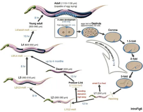
2-3 Life cycle ofC. elegansat 22∘C. 0 min is fertilization. Numbers in blue
along the arrows indicate the length of time the animal spends at a certain stage. First cleavage occurs at about 40 min. postfertilization. Eggs are laid outside at about 150 min. postfertilization and during the gastrula stage. The length of the animal at each stage is marked next to the stage name in micrometers (image from [1 41 ]). . . 40
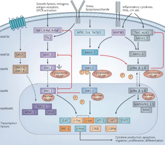
2-4 The three main arms of the mitogen-activated protein kinase (MAPK) pathway, ERK (extracellular signal-regulated kinase), JNK (c-Jun N-terminal kinase) and p38 are shown. They mediate immune cell func-tional responses to stimuli through multiple receptors such as chemoat-tractant receptors, Toll-like receptors and cytokine receptors. The three-tiered kinase dynamic cascade leads to activated MAPKs enter-ing the nucleus and triggerenter-ing immediate early gene and transcription factor activation for cellular responses such as cytokine production, apoptosis and migration. Red arrows indicate feedback or crosstalk within the MAPK pathway (image from [59]). . . 56
3-1Node 𝑣 can represent a protein in a protein network. In this example, degree of node 𝑣 is 4 since it’s connected to 4 other proteins. . . 61
3-2 Example of betweenness computation between nodes𝑖and𝑗. Different nodes on the path between 𝑖 and 𝑗 score different amounts depending on the number of shortest paths passing through them. Here, node 𝑎
has a betweenness score of 1
3 since it is on 1of the 3 shortest paths,
while node 𝑏 scores 2
3 since it is on 2 out of 3 paths. . . 62
3-3 Kirchhoff’s current law . . . 63
3-4 Circuit representation of an interactome network. We model an in-teractome network as an electrical circuit, where a node represents a protein and a resistor represents an interaction. The resistance value of a resistor is inversely proportional to the confidence score of the corresponding interaction. . . 67
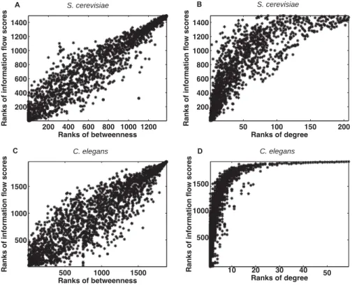
3-5 Scatter plots of ranks of information flow versus betweenness (Panel A) or degree (Panel B) in a S. cerevisiae interactome network and in a C. elegans interactome network (Panel C and Panel D). Overall, ranks of information flow and betweenness are correlated, but a given betweenness usually corresponds to a wide range of information flow scores. Ranks of information flow and degree are less correlated. Low degree can correspond to low, medium or high information flow, but high degree usually corresponds to high information flow. . . 69
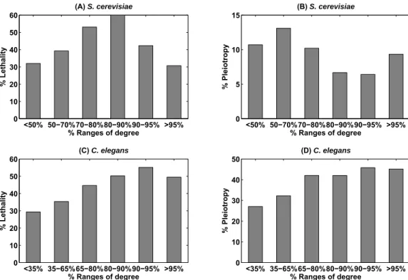
3-6 Correlation between information flow scores and loss-of-function phe-notypes. The higher a proteins information flow score is, the higher the probability of observing lethality (Panel A) or pleiotropy (Panel B) when the protein is deleted from S. cerevisiae. This trend is observed forC. elegansas well (Panel C and Panel D). The correlation is not as strong for betweenness and loss-of function phenotypes. The PCCs for information flow scores and phenotypes are 0.84, 0.60, 0.95, and 0.85 in Panels A-D, respectively. In contrast, the PCCs for betweenness and phenotypes are−0.02, −0.31, 0.67, and 0.49 in Panels A-D, respectively. 71
3-7 Correlation between degree and loss-of-function phenotypes. The higher a proteins degree is, the higher the probability of observing lethality (Panel C) or pleiotropy (Panel D) when the protein is deleted fromC. elegans. However, this trend is not observed for S. cerevisiae (Panel A and Panel B). The PCCs for degrees and phenotypes are 0.31, −0.53, 0.96, and 0.97 in Panels A-D, respectively. . . 72
3-8 Correlation between information flow scores and loss-of-function phe-notypes among proteins of low betweenness. Even among those pro-teins that rank in the lower 30% in terms of betweenness, a propro-teins information flow score is still a good indicator for the probability of observing lethality (Panel A) or pleiotropy (Panel B) when the protein is deleted from S. cerevisiae. This trend is observed for C. elegans as well (Panel C and Panel D). The PCCs for information flow scores and phenotypes are 0.89, 0.79, 0.69, and 0.65 in Panels A-D, respectively. 74 3-9 Correlation between information flow scores and loss-of-function
phe-notypes among proteins of low or medium degrees. Even among pro-teins of low or medium degrees, a propro-teins information flow score is still a good indicator for the probability of observing lethality (Panel A) or pleiotropy (Panel B) when the protein is deleted from S. cerevisiae. This trend is observed for C. elegans as well (Panel C and Panel D). The correlation is not as strong for betweenness and loss-of function phenotypes. The PCCs for information flow scores and phenotypes are 0.80, 0.86, 0.84, and 0.80 in Panels A-D, respectively. In contrast, the PCCs for betweenness and phenotypes among low- or medium-degree proteins are 0.61, 0.037, 0.32, and 0.49 in Panels A-D, respectively. . 75 3-10 Examples of proteins showing high information flow but low
between-ness in theC. elegansinteractome network. The interactions in theC. elegans interactome do not have numerical confidence scores, and the discrepancy between information flow scores and betweenness is likely to be due to topological features such as the existence of alternative paths. KLC-1(Panel A) and TAG-246 (Panel B) are two worm pro-teins that have only 4 interactions, and neither of them scores high in betweenness. However, KLC-1rank the highest 37% and TAG-246 rank in the highest 26% in terms of the information flow scores. The two proteins both correspond to lethal phenotypes upon loss-of-function. 76
3-11 Scatter plots for ranks of information flow scores in different versions of yeast interactome networks (Panel A and C) and for ranks of between-ness in different versions of yeast interactome networks (Panel B and D). The Y-axis represents the rank of information flow scores (Panel A and C) or the rank of betweenness (Panel B and D) in a yeast inter-actome that includes high-confidence interactions only (socio-affinity scores of 4.5 or higher). In Panel A and Panel B, the X-axis represents the rank of information flow scores or the rank of betweenness in a yeast interactome that includes interactions at lower confidence levels (socio-affinity scores of 3.5 or higher). The PCCs for the ranks of infor-mation flow scores (Panel A) and the ranks of betweenness (Panel B) are 0.83 and 0.71, respectively. In Panel C and Panel D, the X-axis rep-resents the rank of information flow scores or the rank of betweenness in a yeast interactome that includes interactions at still lower confidence levels (socio-affinity scores of 2.5 or higher). The PCCs for the ranks of information flow scores (Panel C) and the ranks of betweenness (Panel D) are 0.54 and 0.38, respectively. . . 78
3-12 Muscle-enriched genes identified by semi-supervised analysis. Each row represents a gene and each column represents a tissue or cell type. The normalized values of gene expression are represented in a color scale. Genes are sorted by probability scores (𝑃𝑖) which indicate expression
enrichment in muscle as compared to other tissues. Altogether 310 muscle enriched genes (𝑃𝑖 ≥0.5) were identified. In this plot, the 310
muscle enriched genes, 155 randomly selected genes, and 155 genes with the lowest𝑃𝑖are shown. The list of genes can be found in Appendix B.3
3-13 An interactome network for muscle-enriched genes. We identified direct interacting partners for the muscle-enriched genes from theC. elegans
interactome dataset. We required that an interacting partner must be expressed in muscle cells according to the SAGE dataset. The muscle-enriched genes and their interacting partners form a network. The blue nodes represent the top 20 genes with the highest information flow scores given that the information flow score is calculated just in the muscle network and that the weight of an interaction is defined as the product of the probability scores of the two interacting genes. The green nodes represent the top 20 genes in the muscle network with the highest information flow scores given that the information flow score is calculated in the entireC. elegansinteractome network and that the interactions are unweighted. Some genes (red nodes) rank in the top 20 under both conditions. . . 81
3-14 An interactome network can be partitioned into subnetworks by re-cursively removing proteins of high information flow scores. Panel (A) shows our procedure for network partition, and Panel (B) shows a toy example. . . 88
4-1The Bayesian score compares the hypotheses that the data was gener-ated by one of two distributions. x is a vector of features (a row in a gene table) representing a given item e.g. gene. . . 94
4-2 ROC curves showing the similarity among spatial localization of genes genetically interacting with the same partner. 11 graphs correspond to 10 signaling and 1 DNA-damage response genes used as a background for determining their genetic partners. A fraction of genetic partners were used as a seed for a cluster and the remaining genes were scored on how similar they are to the genes in the cluster and then checked whether they genetically interact with the same partner gene. The number of positives ranges from 27 to 80 (median 52) and negatives from 143 to 282 (median 238). . . 98
4-3 ROC curves showing the similarity among phenotypes resulting from knocking down genes genetically interacting with the same partner. 11 graphs correspond to 10 signaling and 1 DNA-damage response genes used as a background for determining their genetic partners. A fraction of genetic partners were used as a seed for a cluster and the remaining genes were scored on how similar they are to the genes in the cluster and then checked whether they genetically interact with the same partner gene. The number of positives ranges from 45 to 174 (median 97) and negatives from 186 to 467 (median 374). . . 1 00
4-4 Two alternative hierarchical probability models proposed for mod-eling continuous data. (a) Each experimental condition is modeled by a Gaussian: 𝑁(𝑥;𝜇, 𝜎2) with the conjugate
normal-scaled-inverse-gamma prior on 𝜇 and 𝜎2 (joint distribution) (b) Each experimental
condition is modeled by a Gaussian: 𝑁(𝑥;𝜇, 𝜎2) with the conjugate
4-5 Distribution of Bayesian set scores depends on the model. (a) Model variant 1: Distribution of scores based on a query set consisting of two samples (blue) shows the maximum score shifted away from the mean of the two query points; however, it is also away from the mean of the background distribution. (b) Model variant 2: Mean and variance are not coupled together, allowing the Bayesian score to maximize at the mean of the query set distribution. . . 1 05
4-6 ROC curves showing the similarity of microarray profiles of germline genes that genetically interacting with the same partner (using Bayesian sets variant 2 algorithm from Section 4.2.2). 11 graphs correspond to 10 signaling and 1 DNA-damage response genes used as a background for determining their genetic partners. A fraction of genetic partners were used as the input query and the remaining genes were scored on how similar they are to query genes and then checked whether they ge-netically interact with the same partner gene as the query genes. The number of positives ranged from 20 to 64 (median 31) and negatives from 81 to 226 (median 1 85). . . 1 1 0
4-7 (a) ROC based on microarray timecourse during embryonic and lar-val stages for genetic interactors of bar-1, 𝐴𝑟𝑒𝑎𝑅𝑂𝐶 = 0.62, sample
count:50(+),201(−). (b) Genetic interactors of bar-1 constrained to
those which are germline-intrinsic,𝐴𝑟𝑒𝑎𝑅𝑂𝐶 = 0.78, sample count:6(+),13(−).
(c) Genetic interactors ofbar-1constrained to those which are enriched in sperm or oocyte, 𝐴𝑟𝑒𝑎𝑅𝑂𝐶 = 0.93, , sample count:5(+),20(−).
(a)-(c) used Bayesian sets variant 2. (d) Genetic interactors of bar-1 con-strained to those which are enriched in sperm or oocyte using variant 2,𝐴𝑟𝑒𝑎𝑅𝑂𝐶 = 0.82, sample count:5(+),20(−). . . 1 1 3
4-8 Bayesian sets algorithm variant 1applied to group genetic interactors of glp-1 based on their (a) microarray aging data, 𝐴𝑟𝑒𝑎𝑅𝑂𝐶 = 0.67,
sample count:66(+),208(−), (b) microarray aging and heatstress data,
𝐴𝑟𝑒𝑎𝑅𝑂𝐶 = 0.70, sample count:51(+),169(−), (c) microarray aging
and heatstress datasets, considering only sperm- or oocyte-enriched genes,𝐴𝑟𝑒𝑎𝑅𝑂𝐶 = 0.75, sample count:15(+),38(−), (d) microarray
ag-ing/heatstress datasets considering only germline-intrinsic genes,𝐴𝑟𝑒𝑎𝑅𝑂𝐶 =
0.90, sample count:8(+),13(−). . . 1 1 6
4-9 (a) glp-1 genetic interactors grouped by their hypoxia microarray re-sponse, 𝐴𝑟𝑒𝑎𝑅𝑂𝐶 = 0.53, sample count:63(+),218(−), (b) with
ad-ditional constraint of being an oocyte-enriched genes, 𝐴𝑟𝑒𝑎𝑅𝑂𝐶 = 1 ,
sample count:6(+),4(−). . . 1 1 7
4-10 (a)ROC showing the results of running Bayesian sets variant 2 on ge-netic interactors oflet-23described by their microarray profiles during oxidative stress (hypoxia),𝐴𝑟𝑒𝑎𝑅𝑂𝐶 = 0.6, sample count:82(+),500(−)
(b) Constraining the genes in (a) to only those that are annotated as germline-intrinsic, 𝐴𝑟𝑒𝑎𝑅𝑂𝐶 = 0.8, sample count:8(+),29(−). . . 1 1 9
5-1Plots of cosine similarity scores versus Pearson correlation scores for pairs of experiments (each experiment is profiled across genes) of the following types: (a) 25 phenotypes are compared to themselves, 11 ge-netic interaction experiments, 38 localization, 135 microarray; (b) 11 genetic interaction experiments are compared to themselves, pheno-types, spatial localization, and microarray. . . 1 34
5-2 Examples of ROC curves for predicting phenotypes using residual vari-ants 1,2,3. (a) ROC curve for predicting “dumpy” phenotype based on the remaining datasets results in areas under ROC of 0.83, 0.80, and 0.83, for residual variants 1-3, respectively. (b) ROC curve for predict-ing “sterile progeny” phenotype based on all the other datasets results in areas under ROC of 0.87, 0.81, and 0.86, for residual variants 1-3, respectively. . . 1 39
5-3 Plots of predicted versus actual microarray values based on all other datasets using collaborative filtering; 7 randomly selected experiments out of 135 are shown (color corresponds to values for a single experi-ment) with 30 genes predicted per experiment. The legend shows the resulting correlation between the actual and predicted values (a) Re-sults from running factorization-based method of CF (b) Neighborhood-based CF results for the same set of 7 experiments (same color reserved for each experiment). . . 1 42
5-4 Plots of predicted versus actual microarray values based on other mi-croarray datasets using collaborative filtering; 7 randomly selected ex-periments out of 135 are shown (color corresponds to values for a sin-gle experiment) with 30 genes predicted per experiment. The legend shows the resulting correlation between the actual and predicted val-ues (a) Results from running factorization-based method of CF (b) Neighborhood-based CF results for the same set of 7 experiments (same color reserved for each experiment). . . 1 43
5-5 ROC curves illustrate the performance of collaborative filtering for predicting phenotypes based on combined array of other datasets. We selected 12 phenotypes out of 25 at random. For cross validation, 15 positive and 15 negative samples were withheld and predicted based on the remaining data. The results shown here are using factorization-based and neighborhood-factorization-based CF. The areas under the ROC varies from 0.55 to 0.90 for factorization-based estimate (mean 0.72) and from 0.35 to 0.98 for neighborhood based estimate (mean 0.66). . . 1 45
5-6 ROC curves illustrate the performance of collaborative filtering for pre-dicting genetic interactions based on combined array of other datasets. Each of the 11 graphs shows the results of predicting genetic partners for one of the mutant genes used as a background. For cross validation, 15 positive and 15 negative samples were withheld and predicted based on the remaining data. The results shown here are using the global factorization-based estimate. The area under the ROC varies from 0.65 for let-23to 0.96 for let-756 with a mean area under the ROC of 0.81. 147
5-7 ROC curves illustrate the performance of collaborative filtering for predicting genetic interactions based only on the phenotypic data con-sisting of 25 experiments. Each of the 11 graphs shows the results of predicting genetic partners for one of the mutant genes used as a background. For cross validation, 15 positive and 15 negative samples were withheld and predicted based on the remaining data. The results shown here were obtained with factorization-based CF. The area under the ROC varies from 0.56 for sem-5 to 0.94 for let-756 with a mean area under the ROC of 0.73. . . 1 48
5-8 The average area under the ROC curve for predicting genetic interac-tors of 11 mutant genes versus factorization order. The dashed lines correspond to a choice of factor order that would be sufficient to de-scribe the data. For factorization-based CF, 𝑓 = 14 with average area under ROC of 0.77. For neighborhood-based CF, 𝑓 = 6 with average area under ROC of 0.68. . . 1 49 5-9 Conceptual image of how CF can assess how useful a given dataset 𝑛
is for predicting dataset 𝑑 by running the CF prediction for entries in
𝑑 with one input dataset𝑛 at a time. . . 1 51
6-1Maximum margin linear classifier with an offset parameter along with the support vectors (circled); image from [57]. . . 1 55 6-2 ROC curve for predicting genetic interactions using SVM with RBF
kernel of width 0.3. The average area under the ROC curve is 0.92 for 𝐷, 0.86 for 𝑃𝑓=14, 0.83 for entries filled in with zeros and 0.82 for
entries filled with means. The fraction of correctly classified pairs is 0.85, 0.80, 0.74, and 0.73, respectively . . . 1 65 6-3 ROC curve for predicting genetic interactions involving kinases in MAPK
pathway using SVM. The fraction of correctly classified pairs for𝐷and
𝑃𝑓=14 is 0.93 and 0.90, respectively . . . 1 66
6-4 The plots compare how well SVM performs when data is increasingly sparse (from 40% of data missing to 98% of data missing). Prior to classification, the missing values are filled with either collaborative filtering, zeros, or means. . . 1 68
A-1MCC coefficient for nodes 𝑣 and 𝑤 weights in on the number of the mutual neighbors between these two nodes. . . 1 80
B-2 Graph showing the fraction of subnetworks that we found are enriched with GO annotations given specific minimum and maximum subnet-work size thresholds. . . 1 88
List of Tables
3.1Genes in the S. cerevisiae interactome that rank the highest 30% by information flow and rank the lowest 30% by betweenness. . . 73 3.2 Genes showing significant difference of information flow in the muscle
interactome network and in the entire interactome network. The nor-mal motility of the rrf-3 strain is 99±8 thrashes per minute. Genes with * show significantly lower motility rates upon RNAi treatment compared to therrf-3 strain . . . 84 4.1Genes in C. elegans enriched in sperm and oocyte grouped based on
microarray profiles and that genetically interact withbar-1 (all 5 listed) 114 4.2 glp-1interacting germline-intrinsic genes inC. eleganssuccessfully group
by their aging and heatstress microarray profiles, 4 of 8 shown. . . 1 1 5 4.3 glp-1interacting oocyte genes inC. eleganssuccessfully group by their
microarray profiles monitoring their response to oxydative stress (hy-poxia), all 6 shown. . . 1 1 8 6.1Comparing cross validation performance with different SVM kernels
(using full input matrix𝐷with missing entries estimated by𝑃𝑓=14𝑄𝑇𝑓=14).163
6.2 Comparing cross validation performance with different SVM kernels (using 𝑃𝑓=14 as input feature matrix describing genes). . . 1 63
B.1Fraction of modules enriched in GO annotations for a given pair of min/max thresholds. . . 1 89
Chapter 1
Introduction
D. Vasilyev (when asked about𝐻∞norm): Girls, are you ready for a journey? - 6.336 office hours, 2003, unpublished
1.1 Motivation & Objectives
Our research objective is the development of computational methods to predict prop-erties of genes based on other types of biological data. Being able to predict gene properties and experiment outcomes computationally can save large amounts of time and money associated with performing laboratory work. We adapt and extend ex-isting new machine learning algorithms, develop new network metrics, and apply statistical techniques to extract biologically relevant features from various types of high-throughput experimental data. We are particularly interested in identifying gene pairs that genetically interact. Genetic interaction is a broad term referring to a re-lationship between two genes where a simultaneous mutation in both results in an observable joint effect on an organism. This effect is significantly more pronounced or altogether different from individual mutations in either gene.
We focus our research on the genes and pathways involved in the organism’s de-velopment and other core cellular processes. For example, kinases involved in MAPK pathways regulate various cellular activities including gene expression, differentiation, mitosis, cell survival and apoptosis. Mutations in developmental genes are known
to be responsible for a large percentage of cancers, e.g. MAPK kinase cascade is relevant to Hodgkins disease. There are several reasons why we expect genetic in-teractions to occur more frequently within such processes. First, genes involved in development and survival tend to be very important to viability of an organism yet knockouts of a large portion of these genes do not result in observable phenotypes. The event of lacking phenotypes in the face of a genetic mutation is called genetic robustness. We speculate, based on known developmental pathways (e.g. vulval path-way in Caenorhabditis elegans), that this might be due to the fact that biologically important genes are buffered by other functionally overlapping genes or alternative pathways. We hypothesize that such pairs or groups of genes act in a synergistic manner during development (a category of genetic interactions, see Section 1.2) and only deletion of both results in a detectable defect. By identifying pairs of genes that genetically interact, we can provide new information about their function and identify new components of developmental pathways or new pathways altogether. Developmental pathways and genes tend to be more conserved than average, and we can expect to find orthologous relationships in seemingly very different organisms. Therefore, by discovering genetic interactions, we can get better functional maps of various organisms. The majority of our computational analysis has been performed onCaenorhabditis elegans since this model species is relatively well-covered by high-throughput datasets.
1.2 What are genetic interactions?
Genetic interaction between two genes is present when two mutations have a combined effect which is not exhibited by either mutation alone. It is a powerful method for establishing which genes are functionally linked [66, 74, 30, 81]. Genetic interactions are thought to underlie buffering and directly contribute to genetic robustness of an organism [49, 44]. For example, perturbation of a single gene may be buffered by functionally overlapping genes or alternative pathways, as shown in Figure 1-1. In the first scenario, a mutation in both genes would cause lethality. Finding such pairs
can be very useful for cancer research as targeting a gene that is synthetic lethal to a cancer-relevant mutation should kill only cancer cells and spare normal cells [64]. In the second scenario in Figure 1-1 two genes belong to the same pathway. A mutation in one gene partially disables the pathway but does not exhibit a phenotype. Only when both genes are missing, the effect is lethality. In an alternative scenario, one gene may act as a suppressor of another. Knocking down the suppressor gene may result in an observable phenotype, while knocking down both genes results in a wildtype - an organism which seems unaffected phenotypically. An example of that is a pair of genes daf-2 and daf-16 involved in C. elegans dauer formation. Mutation in daf-2
gene causes non-conditional arrest at the dauer stage. Additional mutation indaf-16
gene suppresses daf-2 mutants resulting in a wildtype phenotype [41].
In summary, there is more than one type of genetic interactions: synthetic-lethal interactions in which mutations in two nonessential genes are lethal when combined; suppressor interactions, in which one mutation is lethal but when combined with a second, cell viability is restored; and other more subtle effects such as nonlethal phenotype enhancement and epistasis.
Figure 1-1: Potential mechanisms behind synthetic lethal interaction (image from [30]).
1.3Prior research on genetic interactions and
bi-ological networks
Knowledge of the network of genetic interactions could guide us in discovery of new regulatory and transcriptional mechanisms. It can help us identify functions of pre-viously uncharacterized genes. It can point us to the more subtle pathways. For example, a synergistic effect of a pair of genes may indicate that they form two alter-native branches of a pathway or act in parallel pathways.
The number of possible gene pair combinations to be tested for genetic interac-tions is very large, in the order of 1.8∗108(assuming approximately 19,000 genes inC. elegans). Despite the progress in high-throughput techniques, it would be impossible to systematically test all pairs of genetic interactions. Based on the current estimates, genetic interactions are a very small fraction (less than half a percent [74]) of all pair-wise combinations of genes. Thus, some attempts have been made to computationally predict likely candidate pairs which may interact [127, 139, 66, 153, 98, 24, 70]. Com-putational prediction relies on trying to infer how informative are different gene/pair characteristics for in-silico detection of interactions.
1.3.1 Hypothesized properties of genetically interacting pairs
In an attempt to predict new genetic interactions, several papers in recent years have analyzed properties of known interacting genes. Most of the hypotheses regarding genetic interactions are based on statistical properties of gene data in three model organisms: S. cerevisiae, C. elegans, and D. melanogaster, primarily because these species are among the best studied with the largest amount of high-throughput data available and the largest, albeit still relatively small, number of genetic interactions discovered experimentally.
Lehner et al. [74] performed a statistical network analysis of C. elegans interac-tome and concluded that genes acting as hubs (having many interacting partners) are more likely to engage in genetic interactions. They coined the term ’modifier’ gene
to describe a genetic hub and ’specifier’ gene for its less connected genetic partner. By combining the protein-protein interaction data with phenotypic data, they found that the ’modifier’ hub gene frequently enhances the phenotype of the ’specifier’ low degree gene. Thus, they hypothesize that testing the hub genes and their interacting partners can be more effective than selecting pairs of genes at random. Similarly, Davierwala et al.’s [23] analysis of the essential genes in yeast showed that they are more likely to be involved in genetic interactions than nonessential genes, especially with genes which share similar Gene Ontology annotations. Ozier et al. [99] also showed that pairs of physically linked genes, where one or both exhibit high degree of physical interactions, are substantially more likely to genetically interact than a pair of low physical-interaction degree genes.
Tong et al. [127] found that genetic interactors in yeast tend to share similar phe-notypes, subcellular location, and are often part of the same protein complex. More-over, they found that network motifs built of interactions can be used for predicting new ones. Network analysis approach to discover patterns of genetic interactions has also been pursued in yeast by Bader et al. [5], who found that genetically interacting genes tend to be in a closer proximity in protein-protein network than a random pair of genes, and that a combination of physically and genetically interconnected proteins forms functional complexes.
It is interesting to note that there are claims of differences between yeast and
C. elegans genetic interaction networks. In yeast, Kelley and Ideker [66] found that genetic interactions are significantly more enriched between genes belonging to dif-ferent pathways (3.5 times more likely) rather than between those within the same pathway. That is, they are more likely to belong to redundant or complementary pro-cesses than to partake in the same process. In C. elegansLehner et al. [73] claim the opposite. They state that within-pathway interactions are twice as likely to happen than between-pathway interactions. It is difficult to establish at this point whether the difference is due to system-level biological differences between the organisms or the methods that have been used to discover genetic interactions known to date.
homology studies of gene sequences could pinpoint genetic interactors. Several studies have been done to identify such classes of duplicated genes [126, 132], and we now know that only a small portion (less than 2%) of known synthetic lethal pairs encode homologous proteins.
1.3.2 Current computational approaches to identify genetic
interactions
In the previous section we discussed several gene pair properties that have been linked to genetic interactions. As of now, all of the above characteristics can be classified as ’weak’ predictors of genetic interactions. Current computational approaches attempt to combine results from multiple ’weak’ indicators to predict genetic interactions. They can be grouped into three broad categories:
1. Using local network properties in physical and genetic protein networks to pre-dict new interactions.
2. Integrating different kinds of genomic datasets to predict new genetic interac-tions.
3. Using interactions from various species to predict interactions in related species.
Predicting genetic interactions with network structures
To predict genetic interactions, Tong et al. [127] explored the ’small world’ property of genetic interaction networks in yeast. They discovered that if two genes share a genetic interaction with a common partner, they are likely to interact with one another. In ∼ 20% of cases the neighbors of a query gene could also interact with each other in comparison to less than 1% of random gene pairs.
As mentioned previously, Lehner et al. [74] concluded that high degree genes and their partners are more likely candidates for genetic interactions than a randomly selected pair. Subsequently, they used their finding to predict and test for more interactions.
Predicting genetic interactions by integrating different types of genomic data
Different types of genomic data have been shown to be weak indicators of genetic interactions (see Section 1.3.1) but their predictive power can increase if combined together. Wong et al. [139] used decision trees to integrate protein localization, mRNA expression, physical interaction, known function and network topology data in order to predict synthetic lethal or sick interactions in yeast. Cross validation tests showed that while using a single source of evidence resulted in a slight improvement in per-formance over random, combining several evidence sources led to significantly better specificity/sensitivity. They tested a subset of their predictions and found that 49 out of 318 could be verified as opposed to 2 they would expect by chance.
Bayesian integration has been another popular approach used to integrate different types of functional data. Using this approach, genetic interactions have been predicted for approximately 10% ofC. elegansgenes, using information on expression patterns, phenotypes, functional annotations, microarray coexpression, and protein interactions [58, 69, 129, 153, 121].
Predicting genetic interactions using orthology
Genetic interactions identified in one species can be experimentally tested in second species if the genes participating are orthologues in both genomes. Tischler et al. [126] took more than 1000 synthetic lethal interactions in yeast and tested their orthologues inC. elegans. They found that only a very small subset (less than 1%) is conserved. This is in contrast to mutations in single genes where more than 60% of essential genes in yeast have essential orthologues in C. elegans [65]. It leads to the following theory: for synthetic lethal interactions, it matters whether the organism is unicellular or multicellular. However, even a weak indicator such as genetic pair orthology can be useful in future studies, if combined with other features.
Despite the progress in computational methods tackling genetic interaction pre-diction, the incompleteness and sparsity of available data along with a lack of decisive
features, provide for a challenging problem.
1.4 Thesis summary
In this thesis, we present machine learning and other computational approaches we developed and/or adapted to biological data with a goal of predicting genetic interac-tions inC. elegans. In this Chapter, we described genetic interactions and the current approaches aimed at predicting them computationally. The remainder of the thesis is structured as follows:
Chapter 2 describes the relevant biological background, starting with an overview of the two model organisms studied: Caenorhabditis elegansandSaccharomyces cerevisiae. Next, we describe the experimental datasets and features extracted from these datasets, both of which are inputs to our learning algorithms in the subsequent chapters. Finally, we conclude with an overview of a MAPK pathway that we use in our computational work later.
Chapter 3 introduces a graph-based metric ofinformation flow, which we devel-oped to analyze the importance of a protein in an interactome. We show that the information flow metric is a strong predictor of essentiality and pleiotropy and that it outperforms the established metrics such as betweenness and degree. We further test the performance of the information flow metric in the presence of noise in the data. We also show how information flow can detect important genes in signaling networks with directionality or in networks constrained to specific tissues.
In Chapter 4, we adapt the Bayesian sets method [37] to biological data in order to evaluate the relevance of experimental datasets to predicting genetic interactions. We extend Bayesian sets to enable us to analyze continuous data. Among other conclusions, we assess that while genetically interacting genes do not seem to co-localize, they tend to share similar phenotypes and be up- or down-regulated together during development or aging.
Chapter 5 describes novel use of collaborative filtering (CF) to predict genetic interactions and other experimental data such as phenotypes or microarray expression profiles. We adapt a global factorization-based CF approach and a local neighborhood-based CF approach [13] to handle a mixture of discrete and continuous entries. We use CF to fill in missing values, evaluate how relevant given data is to genetic interactions and to predict genetic interactions.
Our last contribution is predicting genetic interactions with Support Vector Machines [130, 57] as described in Chapter 6. We show that SVM outperforms CF at predicting genetic interactions, and discuss the role of the radial basis function (RBF) kernel. We further show that the performance improves if we narrow down genes to specific functional categories. Finally, we discuss the importance of collaborative filtering which fills in the missing values in the input feature matrix, a necessary condition for successful classification with SVM. We summarize and briefly discuss our contributions in Chapter 7.
Chapter 2
Biology Background
Dad:I tell everyone at work that you work at the White House.
Patrycja: It’s not “White House” dad, it’s “Whitehead”!
Dad, absentmindedly:Right, right, I keep confusing this, sorry.
- Poland, 2007, unpublished
This Chapter introduces relevant biological concepts. First, the Chapter cov-ers some of the biological properties of the organisms studied, more specifically
Caenorhabditis elegansandSaccharomyces cerevisiae, in order to elucidate what kinds of data we can expect to have for analysis as well as what types of questions we can explore. Next, we describe the individual datasets in more detail, and briefly discuss the types of information we plan to extract from each of these datasets.
2.1
Caenorhabditis elegans
as a model organism
Caenorhabditis elegans [53] is a small nematode (worm) that lives in the soil across most of the temperate regions of the world. Since it requires only humid environment, ambient temperature, oxygen, and bacteria as food, it is very cheap and easy to maintain in the lab. C. elegans are grown on agar plates or in a liquid culture with E. coli as a food source. The adults are on average 1mm long and require a microscope for handling. C. elegans exhibit no smell and are transparent. The worm life cycle, from an egg to an adult producing more eggs, takes 3.5 days at 20 degrees Celsius. There are two sexes, male and hermaphrodite which differ in both
appearance and in frequency. A hermaphrodite produces both sperm and oocytes and can reproduce by self-fertilization (see Figure 2-1). A male produces only sperm thus it must mate to produce offspring (see Figure 2-2). X0 males arise spontaneously in XX hermaphrodite populations by means of X chromosome nondisjunction at a frequency of approximately 0.1%. Hermaphrodite lays about 300 eggs during its reproductive life. If it mates with a male, it can produce as many as 1000 eggs with a ratio of 1:1 of male and hermaphrodite cross progeny. Additionally, it would produce hermaphrodites by selfing.
Figure 2-1: Anatomy of an adult hermaphrodite. A. DIC image of an adult hermaphrodite, left lateral side. Scale bar 0.1mm. B. Schematic drawing of anatom-ical structures, left lateral side (image from [141])
The life cycle of C. elegansis comprised of the embryonic stage, four larval stages (L1-L4) and adulthood, see Figure 2-3. After the larval stage is over, the worm be-comes fertile in 4 days. Its total lifespan is approximately 2-3 weeks. The life cycle of a worm starts when mature oocytes pass through the spermatheca and become fertilized either by sperm from a hermaphrodite or a male. Within 30 minutes after fertilization, the zygote develops a shell and a membrane making the embryo imper-meable to most solutes and able to survive outside the uterus. The eggs are laid at gastrulation, at about 3 hours after fertilization. Embryogenesis consists of 2 phases: 1) cell proliferation and organogenesis, and 2) morphogenesis. During the
prolifera-Figure 2-2: Anatomy of an adult male. A. Anatomical structures, left lateral side. B. DIC image of an adult, left lateral side. Scale bar 0.1mm. C. The unilobed distal gonad. D. The adult male tail, ventral view. Arrow points to cloaca, arrowhead marks the fan. Rays 1-9 are labeled with asterisks on the left side. E. L3 tail, bottom, is starting to bulge (image from [141])
tion phase the precise temporal and spatial pattern of organ formation is followed, giving rise to a fixed number of cells with predetermined fates. This process is fully invariant from one embryo to another. The next stage lasting approximately 7 hours consists of the body changing its shape and neural connections being made. Next, a cuticle is secreted. The L1larva hatches at 14 hours after fertilization. Outside the vulva, the larval development goes through L1-L4 stages punctuated by molts. More cell division takes place, and with the exception of the germline, all cell lineages follow an almost invariant temporal and spatial assignment. The four larval stages are punctuated by molts when the new cuticle is formed under the old one and the old one shed during a brief period called lethargus.
If the food supply is limited in early larval development, C. elegans can take an alternative, a dauer pathway, at the L2/L3 molt to produce a dauer larva, an non-eating alternative to L3 stage that can survive up to 3 months without continuing development. When the food becomes available, the dauer goes into L4 and resumes
normal development.
Figure 2-3: Life cycle of C. elegans at 22∘C. 0 min is fertilization. Numbers in blue
along the arrows indicate the length of time the animal spends at a certain stage. First cleavage occurs at about 40 min. postfertilization. Eggs are laid outside at about 150 min. postfertilization and during the gastrula stage. The length of the animal at each stage is marked next to the stage name in micrometers (image from [141]).
C. elegansis the first multicellular organism to have its genome sequenced (1998)[21]. It is a relatively simple organism, both anatomically and genetically. A complete cell lineage of C. elegans has been mapped and we know that, on the cellular level, each individual develops in an almost identical fashion. The adult hermaphrodite has 959 somatic cells and the adult male has 1031. The genome of C. elegans consists of 108 nucleotide pairs encoding for approximately 19,000 genes. Genes are arranged
on six haploid chromosomes. The haploid set includes five autosomes (A) and a sex chromosome (X), all roughly equal in size. Hermaphrodites are diploid for all six chromosomes (XX), while males are diploid for the autosomes but have only one X chromosome (XO) [140]. The C. elegans genome proves that many biological mech-anisms are conserved across the animal kingdom, and as new vertebrate genes are cloned, frequently one can find a direct C. elegans homologue.
The basic anatomy of C. elegans includes a mouth, pharynx, intestine, gonad, and collagenous cuticle. Males have a single-lobed gonad and a tail specialized for mating. Hermaphrodites have two ovaries, oviducts, spermatheca, and a single uterus. The body plan consists of two concentric tubes separated by a fluid-filled space, the pseudocoelom. Extracellular collagenous cuticle, secreted by hypodermis, covers the outer tube [140]. Body muscles responsible for movement are arranged in four stripes along the length of the animal. The outer tube also consists of the nervous system, gonad, coelomocytes, and excretory/secretory system. The inner tube is composed of a pharynx, pharyngeal nervous and muscular systems and an intestine. Most of the neurons are around the pharynx, along the ventral midline and in the tail. C. elegans moves either forward or backward in a sinusoidal wave using its longitudal body muscles.
Eating and reproduction are the primary focus of C. elegans life. The pharynx grinds and pumps food into the intestine. The intestinal cells line the lumen which connects to the anus positioned near the tail. The hermaphrodite reproductive system consists of functionally independent anterior and posterior arms. Each arm consists of an ovary, vulva, a more proximal oviduct, and a spermatheca connected to a common uterus. The adult uterus contains fertilized eggs and embryos in the early stages of development. To lay eggs, the hermaphrodite contracts its vulval muscles. The male gonad is a single organ. Meiotic cells in progressively later stages of spermatogen-esis are distributed along the gonad and the seminal vesicle. Male-specific neurons, muscles, and hypodermal structures are required for mating.
C. elegans is a popular model organism for high-throughput studies due to its advantages, in summary:
1. A fully sequenced genome.
2. Cell lineages have been fully mapped and shown to be invariant.
3. Easy of maintenance in the lab, requires only bacteria and ambient temperature for growth.
5. Mutant strains can be stored for long periods of time at low temperatures. 6. Self-fertilizes or can be crossed with mutant males.
7. Transparent and odorless, thus easy to handle and spot mutations using the microscope.
8. Receptive to many forms of mutagenesis using chemical mutagens; RNAi via injection, feeding, or soaking is quite effective.
9. Many pathways and genes have orthologous in other species including humans.
2.2
Saccharomyces cerevisiae
as a model organism
Saccharomyces cerevisiae is one of the most intensively studied eukaryotic model organisms in molecular and cell biology. It is a species of budding yeast, reproducing by a division process known as budding. S. cerevisiae cells are round to ovoid, 510 micrometers in diameter.
S. cerevisiaeis popular for studying the cell cycle because it is easy to culture, but, as a eukaryote, it shares the complex internal cell structure of plants and animals. S. cerevisiae was the first eukaryotic genome to be completely sequenced. The genome is composed of about 13∗106 base pairs and 6,275 genes, compactly organized on 16
chromosomes. It is estimated that yeast shares about 23% of its genome with that of humans.
There are two forms in which yeast cells can survive and grow, haploid and diploid. The haploid cells undergo a simple life cycle of mitosis and growth, and under con-ditions of high stress will generally simply die. The diploid cells (the preferential ’form’ of yeast) similarly undergo a simple life cycle of mitosis and growth, but under conditions of stress can undergo sporulation, entering meiosis and producing a variety of haploid spores, which can go on to mate (conjugate), reforming the diploid. Yeast has two mating types, 𝑎 and 𝛼, which show primitive aspects of sex differentiation, and are hence of great interest.
S. cerevisiae is a widely used model organism in science, and, is, therefore, one of the most studied. S. cerevisiae has obtained this important position because of its established use in industry (e.g. beer, bread and wine fermentation, ethanol production). Additionally, yeasts are comparatively similar in structure to human cells, both being eukaryotic, in contrast to the prokaryotes (bacteria and archaea). Many proteins important in human biology were first discovered by studying their homologs in yeast; these proteins include cell cycle proteins, signaling proteins, and protein-processing enzymes. The highly annotated yeast genome [146] makes for an important tool for developing basic knowledge about the function and organization of eukaryotic cell genetics and physiology. S. cerevisiae is also covered by vast amounts of other high-throughput data such as micro arrays, protein interaction networks, signaling networks, knockout experiments etc, making it suitable as a source of addi-tional data. We utilizeS. cerevisiaedata to confirm traits that link properties of genes in interactive and phenotypes as well as provide more complete signaling networks for analysis.
2.3High-throughput datasets
C. eleganshas been studied extensively since its introduction in 1974 by Sydney Bren-ner [19]. Since the species are well-adapted and easy to handle in high-throughput studies, multiple datasets are available covering large portions of or an entire worm genome. Similarly, compared with other species, S. cerevisiae is covered by vast amounts of high-throughput data. In the following sections, we list the categories of experimental data available along with a brief description about each. Within each category, we provide specific information about the datasets relevant to our compu-tational work in the latter chapters.
2.3.1 DNA Microarrays
DNA microarrays are used to quantitatively measure levels of mRNA expression in a collection of cells which can be specific tissues or an entire organism. Microarrays can
be used to identify genes involved in embryogenesis or development by taking genome expression level ’snapshots’ at different timepoints. Microarrays can be also used to study mutations or diseases (e.g. cancer) by comparing gene levels in wildtype versus mutant strains.
We are interested in the nature of gene interactions during the species’ life cycle including embryogenesis, development, adult life and aging. We are also interested in genes involved in the stress response or abnormal function e.g. cancer. Therefore we use data on gene expression levels present across time in either wildtype or mutant strains. This allows us to elucidate the functional relationships between gene pairs: potential suppressors, enhancers etc. We use a compendium of microarray datasets from the worm as listed below:
1. mRNA expression levels of 8890 genes in a wildtype C. elegans strain across 10 timepoints from the first to the fourth hour of embryonic development [9]. 2. mRNA expression levels of 8890 genes in amex-3mutant C. elegansstrain with
skn-3(RNAi) across 10 timepoints from the first to the fourth hour of embryonic development [9].
3. mRNA expression levels of 8890 genes in apie-1mutant C. elegansstrain across 10 timepoints from the first to the fourth hour of embryonic development [9]. 4. DNA microarray data covering 17,871 genes (94% of the C. elegans genome) in
a wildtype worm, representing relative levels of gene expression during devel-opment, from eggs through adulthood, 7 timepoints [62].
5. DNA microarrays containing 11,917 genes in a wildtype population of worms. The worms were synchronized in the L3 larval stage and then RNA was prepared every 2 hours from the 32nd to the 44th hour after hatching for a total of 7 timepoints. This age range spans the entire time from the initial specification of vulval fates to the completion of the vulval lineages (study of vulval cell specification from [110]).
6. DNA microarrays containing 11,917 genes in a let-60 mutant population of worms. The worms were synchronized in the L3 larval stage and then RNA was prepared every 2 hours from the 32nd to the 44th hour after hatching resulting in a total of 7 timepoints (study of vulval cell specification from [110]).
7. DNA microarrays containing 11,917 genes in a let-23 mutant population of worms. The worms were synchronized in the L3 larval stage and then RNA was prepared every 2 hours from the 32nd to the 44th hour after hatching for a total of 7 timepoints (study of vulval cell specification from [110]).
8. In this study of aging and longevity in C. elegans, RNA was isolated from age-synchronized cultures of 17,871 worms at 6 timepoints during their lifespan, starting at the first day of adult life (3 days after fertilization) to an age of 16-19 days at which 90% of the population was dead [79].
9. mRNA expression levels of 18,455 C. elegans genes were measured at 7 time-points during normal adult aging using synchronized populations at 0 hours (young-age adult) to 144 hours (middle-age adult) [84].
10. mRNA expression levels of 18,455 C. elegans genes were measured at 7 time-points in heatstress conditions using synchronized populations at 0 hours (young-age adult) which were cultured at 25∘C, then switched to 30∘C and sampled
over a 12 hour time period [84].
11. DNA microarrays containing 11,990C. elegansgenes were hybridized across 29 total timepoints covering the developmental timecourse among 4 different worm cultures. A mixed stage population of wildtype worms were grown at 20∘C, and
mutant worms were grown at 15∘C in liquid culture (glp-4) or on peptone plates
(fem-1 and fem-3) [107].
12. DNA microarrays containing probes for 17,817C. elegansgenes were hybridized for synchronized populations of wildtype worms under normal conditions (3 timepoints) and under oxidative stress conditions (hypoxia) for synchronized mutants hif-1 (3 timepoints) andvhl-1 (3 timepoints) [116].
13. DNA microarrays containing probes for 17,088C. elegansgenes in synchronized dauer stage worms were examined for gene changes during the transition from dauer into normal development. The worms were fed at 0 hour and then ob-served over a 12 hour period after feeding. They were harvested approximately every 1 hour for a total of 11 timepoints [134].
14. DNA microarrays containing 17,088 C. elegans genes in synchronized starved L1stage. Worms were fed at timepoint 0 and subsequently harvested at approx-imately 1 hour intervals for over 12 hours after feeding (11 timepoints) [134].
2.3.2 Spatial expression patterns
Spatial expression patterns describe where protein products of genes are localized within an organism. This gives us information about the presence or enrichment of proteins in specific types of cells or tissues, e.g. muscle, intestine, neuronal, pharynx. The spatial datasets we use have been obtained using a variety of different methods: 1. Promoter GFP::fusion data - promoters targeting genes of interest are fused with green fluorescent protein (GFP). GFP staining is used to visually localize genes in specific tissues. The output from this method is generally qualitative as it is done by visually screening the organism and indicating where fluorescence is present. The GFP construct needs to be done separately for each individual gene; thus the method’s throughput is low. To date, only a fraction of the C. elegansgenome has been screened. Relevant data we plan to use is a GFP::fusion dataset which covers 1571 genes across 46 spatial locations in larval and adult tissues [125].
2. Serial Analysis of Gene Expression (SAGE) data - SAGE is a technique used to obtain a quantitative snapshot of the mRNA population in a sample of interest. The traditional SAGE approach is based on a principle that a short sequence tag (10-14 base pairs) contains sufficient information to uniquely identify a transcript, provided that that the tag is obtained from a unique position within
each transcript. First, mRNAs are isolated from a sample (e.g. specific tissue) of interest. Then a short (10-14 base pairs) sequence chunk is extracted from each mRNA and these chunks are all linked together to form a long chain. Resulting chains are amplified via a polymerase chain reaction (PCR). Next, they are sequenced and each tag is matched to its corresponding gene. The quantity of tags observed provides information about the expression level of the corresponding gene. We have SAGE data covering more than 14,000C. elegans
genes across 12 specific tissues [86].
3. Spatial data from Wormbase is based on multiple data sources and covers 3394 genes in 38 spatial locations in adult tissues [145].
2.3.3 Phenotypes
A phenotype consists of an organism’s observable properties such as its morphology, development, or behavior. Phenotypic differences between wildtype and mutant ani-mals can be used to link genes to their function in an organism. Various mutagenic treatments have been shown to effectively induce gene mutations in C. elegans. If a single gene knockout is successful and the species viable, the resulting mutant strains are preserved using hermaphrodite libraries. However, keeping mutant strains is te-dious and expensive, and another method to knock down genes has become popular: RNA interference (RNAi).
RNAi is a process of post-transcriptional gene silencing by which double stranded RNA (dsRNA) causes sequence-specific degradation of homogolous mRNA sequences. dsRNA of a desired knock-out gene is introduced into a cell in an attempt to suppress the expression of that gene.
Double mutants created by genetic crossing of different strains are very hard to obtain. Single gene mutant strains are expensive, difficult to control for experimen-tally, and they are primarily hermaphrodites. Males are needed for double mutant crosses. Double RNAi is not nearly as robust as single RNAi and frequently unde-sired off-target effects occur. The most successful approach for double mutant is to
![Figure 1-1: Potential mechanisms behind synthetic lethal interaction (image from [30]).](https://thumb-us.123doks.com/thumbv2/123dok_us/10122711.2912887/29.918.189.733.722.944/figure-potential-mechanisms-synthetic-lethal-interaction-image.webp)