Sparsification and Separation of Deep Learning Layers
for Constrained Resource Inference on Wearables
Sourav Bhattacharya
§and Nicholas D. Lane
§,† §Nokia Bell Labs,†University College LondonABSTRACT
Deep learning has revolutionized the way sensor data are analyzed and interpreted. The accuracy gains these ap-proaches o↵er make them attractive for the next genera-tion of mobile, wearable and embedded sensory applica-tions. However, state-of-the-art deep learning algorithms typically require a significant amount of device and pro-cessor resources, even just for the inference stages that are used to discriminate high-level classes from low-level data. The limited availability of memory, computation, and en-ergy on mobile and embedded platforms thus pose a signif-icant challenge to the adoption of these powerful learning techniques. In this paper, we propose SparseSep, a new ap-proach that leverages the sparsification of fully connected layers and separation of convolutional kernels to reduce the resource requirements of popular deep learning algorithms. As a result, SparseSep allows large-scale DNNs and CNNs to run efficiently on mobile and embedded hardware with only minimal impact on inference accuracy. We experiment using SparseSep across a variety of common processors such as the Qualcomm Snapdragon 400, ARM Cortex M0 and M3, and Nvidia Tegra K1, and show that it allows inference for vari-ous deep models to execute more efficiently; for example, on average requiring 11.3 times less memory and running 13.3 times faster on these representative platforms.
CCS Concepts
•Computing methodologies!Machine learning; Neu-ral networks; •Computer systems organization ! Embedded software;
Keywords
Wearable computing; deep learning; sparse coding; weight factorization
1. INTRODUCTION
Recognizing contextual signals and the everyday activity of users from raw sensor data is a core enabler for mobile and wearable applications. By monitoring user actions (via speech, ambient audio, motion) and context using a variety of sensing modalities, mobile developers are able to provide both enhanced, and brand new, application features. While sensor-related applications and systems are still maturing, and are highly diverse, a notable characteristic is their re-liance on making a wide-variety of sensor inferences. Accurately extracting context and activity information from noisy mobile sensor data remains an unsolved problem. Be-cause the real world is highly complex, unpredictable and constantly changing, it often causes confusion to the ma-chine learning and signal processing algorithms used by
mo-bile devices. One of the most promising directions today in overcoming such challenges is deep learning [1, 2]. De-velopments in this particular field of machine learning have caused the approaches and algorithms used in even mature sensing tasks to be completely changed (e.g., speech [3] and face [4] recognition). The study of deep learning usage for mobile applications is in its early stages (e.g., [5, 6, 7, 8]), but with promising initial results.
While deep learning o↵ers important benefits to robust mod-eling, its integration into mobiles and wearables is compli-cated by the sizable system resource requirements these algo-rithms introduce. Barriers exist in the form of memory, com-putation and energy; these collectively prevent most deep models from executing directly on mobile hardware. Conse-quently, existing examples of deep learning for smartphones (e.g., speech recognition) remain largely cloud-assisted. A number of negative side-e↵ects of this: first, inference ex-ecution becomes coupled to fluctuating and unpredictable network quality (e.g., latency, throughput); but more im-portantly it exposes users to privacy dangers [9] as sensitive data (e.g., audio) is processed o↵-device by a third party. Allowing broaderdevice-centric deep learning classification and prediction will need the development of brand-new tech-niques for optimized resource sensitive execution. Up to this point, the machine learning community has made excellent progress in training-time optimizations and is only now be-ginning to consider how these ideas transfer to inference-time. Currently, most knowledge of deep learning algo-rithm behavior on constrained devices is largely limited to one-o↵ task-specific experiences (e.g., [10, 11]). These sys-tems are limited however is providing examples and evidence that local execution is feasible, although they do provide some insights for ways forward. What is required however is a deeper study of these issues with an aim towards the development of techniques like o↵-line model optimization and runtime execution environments to match the resources (e.g., memory, computation and energy) present on edge de-vices like wearables and mobile phones.
In this work, we make an significant progress into the de-velopment of such algorithms and software by developing a sparse coding- and convolution kernel separation-based approach to optimizing deep learning model layers. This framework – SparseSep – includes: (1) a compiler, Layer Compression Compiler (LCC), in which unchanged deep mod-els are inserted and then optimized; (2) a runtime frame-work, Sparse Inference Runtime (SIR), that is able to exploit the transformation of the model and realize radical reduc-tions in computation, energy and memory usage; and (3) a separator, Convolution Separation Runtime (CSR), that sig-nificantly reduces convolution operations. SparseSep tech-niques can allow a developer to adopt existing o↵-the-shelf
deep models and scale their processor behavior such as, ac-ceptable accuracy reduction and device limits, e.g., memory and necessary execution time.
The core concept of this work is the hypothesis that compu-tational and space complexity of the deep learning models can be significantly improved through the sparse representa-tion of key layers and separarepresenta-tion of convolurepresenta-tion layers. Deep models often have millions of parameters spread throughout a number of hidden layers that capture the robust represen-tations of the data. By using theory from sparse dictionary learning we investigate how the originally complex synap-tic weight matrix can be captured in much smaller matri-ces that require less computational and memory resourmatri-ces. Critically, such theory a↵ords the ability of these sparsified layers to be faithful to the originals with theoretical bounds on important aspects such as, reconstruction error. This is the first time this approach has been used.
Our experiments include both DNNs and CNNs, the most popular forms of deep learning today. Tests span both au-dio classification tasks (ambient scene analysis and speaker identification) that are common in the mobile sensing sys-tems; along with image tasks (object recognition) seen in mobile vision devices like Google Glass. We find that across a range of experiments and devices SparseSep can allow deep models to execute using (on an average) only 26% of the orig-inal energy while only sacrificing approximately up to 5% of the accuracy of these models. Specific examples include the Snapdragon 400 processor running a deep learning model for speaker identification with a 4.1 times improvement in exe-cution time, and a 17.6 times reduction in memory. Further-more, we benchmark this deep learning version of speaker identification and find, as expected, that the deep model is much more robust than models conventionally used (such as random forests). Most important of all, we examine de-vice restrictions found on other common processors like the Cortex M3 equipped with 32 KB of RAM. Not surprisingly we find these processors can not support any form of deep learning model tested (due to restrictions to computation and/or memory) –until we apply the SparseSep process. The key scientific contributions of this research are:
• We propose, for the first time, a sparse coding-based approach to the optimization of deep learning inference execution. We propose the use of convolution kernel sep-aration technique to minimize overall computations of CNNs on resource constrained platforms.
• To our knowledge, this work is the first to demonstrate very deep learning models (many layer DNNs and CNNs) executing on severely constrained wearable hardware with acceptable levels of performance (energy efficiency, com-putation times).
• We design and implement a prototype that realizes our approach to sparse dictionary learning and kernel sepa-ration into deep learning model representation and infer-ence execution. We implement necessary runtime com-ponents for 4 embedded and mobile processor platforms.
• We experiment with four di↵erent CNN and DNN mod-els under large audio and image datasets. We demon-strate gains of the order of 11.3⇥improvements in mem-ory and 13.3⇥in execution time under multiple exper-iment configurations, while only su↵ering accuracy loss of⇡5%.
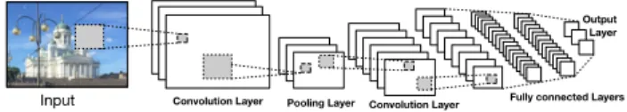
Input Pooling Layer Fully connected Layers Convolution Layer
Output Layer
Convolution Layer
Figure 1: A CNN mixes convolutional and feed-forward layers
2. BACKGROUND
Popular deep learning architectures, such as Restricted Bo-ltzmann Machines and Deep Belief Networks, share a com-mon architecture. Often, they are collectively referred to as Deep Neural Networks. Typically, a DNN contains a num-ber of fully-connected layers, where each layer is composed of a collection of nodes. Sensor measurements (e.g., audio, images) are fed to the first layer (the input layer). The fi-nal layer, also known as the output layer, corresponds to inference classes with nodes capturing individual inference categories (e.g., music or cat). Layers in between the input and the output layer are referred to as hidden layers. The degree of influence of units between layers vary on a pair-wise basis determined by a weight value. Together with the synaptic connections and inherent non-linearity, the hidden layers transform raw data applied to the input layer into the prediction classes captured in the output layer.
DNN-based inferencing follows a feed-forward algorithm that operates on sensor data segments in isolation. The algorithm starts at the input layer and moves layer wise sequentially, while updating the activation states of all nodes one by one. The process finishes at the output layer when all nodes have been updated. Finally, the inferred class is identified as the class corresponding to the output layer node with the great-est state value.
CNNs are another popular class of deep models that share architectural similarities to DNNs. As presented in Fig-ure 1, a CNN model contains one or more convolutional layers, pooling or sub-sampling layers, and fully connected layers (equivalent to those used in DNNs). The objective of these layers is to extract simple representations from the in-put data, and then converting the representation into more complex representations at much coarser resolutions within the subsequent layers. For instance, first convolutional fil-ters (with small kernel width) are applied to the input data to capture local data properties. Next, max or min pooling is applied to make the representations invariant to transla-tions. Pooling operations can also be seen as a form of di-mensionality reduction. Lastly, fully connected layers (i.e., a DNN) help a CNN to make predictions.
A CNN follows a sequential approach, as in DNNs, to gener-ate isolgener-ated prediction at a time. Often in CNN-based pre-dictions, sensor data is first vectorized into two dimensions. Next, data is passed through a series of convolution, pooling and non-linear layers. The purpose of the convolution and pooling layers can be viewed as that of feature extractor be-fore the fully connected layers are engaged. Inference then proceeds exactly as previously described for DNNs until ul-timately a classification is reached.
Contrary to the shallow learning-based models, deep learn-ing models are usually big an often contains more than mil-lion parameters. High parameter space improves the capac-ity of these models and they often outperform prior shallow models in terms of model generalization performances. How-ever, the accuracy gains come at the expense of high energy
and memory costs. Although, high end wearables contain-ing GPU, e.g., NVIDIA Tegra K1, can efficiently run deep models [12], the high resource demands make deep learning models unattractive for low end wearables. In this paper we explore sparse factorizations and convolutional kernel sep-arations to optimize the resource demands of deep models, while maintaining the functional properties of the models.
3. DESIGN AND OPERATION
Beginning with this section, and spanning the following two, we detail the design and algorithms of SparseSep.
3.1 Design Goals
SparseSep is shaped on the following objectives.
• No Re-training. The training of a large deep model is the most time consuming and computationally demand-ing task. For example, a large model such as GoogleNet is trained using thousands of CPU cores [13], which is beyond the current capabilities of a single wearable de-vice. In this work, we mainly focus on the inference cycle of a deep model and perform no training on the resource-constrained devices. The training process also requires a very large training dataset, often inaccessible to the developers [14]. Thus new techniques are needed to compress popular cloud-scale deep learning models to run on wearable and IoT grade hardware gracefully.
• No Cloud O✏oading. As noted in §1, o✏oading the execution of portions of deep models can result in leaking sensitive sensor data. By keeping inference com-pletely local, user and applications have greater privacy protection as the data or any intermediate results never leave the device.
• Target Low-resource Platforms. Even high-end mobile processors (such as the Tegra K1 [15]) still require careful resource use, when executing deep learning mod-els. But in this class of processors, the gap in resources is closing. However, for low-energy highly portable wear-able processors that lack GPUs or have only a few MBs of RAM (e.g., ARM Cortex M3 [16]), local execution of deep models remains impractical. For this reason, Spars-eSep turns to new ideas like the use of sparsification of weights and kernel separation, in search of the leaps in resource efficiency required to make these low-end pro-cessors viable.
• Minimize Model Changes. Deep models must un-dergo some degree of change to enable their operation on wearable hardware. However, a core tenet of Spars-eSep is to minimize the extent of such modifications and remain functionally faithful to the initial model ar-chitecture. For this reason, we frame the problem as one of deep model compression (originally formulated by the machine learning community), where model layer ar-rangements remain unchanged and only per-layer con-nections are changed through the insertion of additional summarizing layers. Thus, the degree of changes made by SparseSep is a key metric that is minimized during model processing.
• Adopt Principled Approaches. Ad-hoc methods to alter a deep model – such as ‘specializing’ a model to recognize a smaller set of activities/contexts, or chang-ing layer/unit parameters to generate a desired resource
consumption profile – are dangerous as they violate the domain experience of the modeling experts. Methods like sparse coding [17] and model compression [18] are sup-ported by theoretical analysis [19]. Assessing if a model can be altered solely by changes in the accuracy metric can be dangerous and can potentially hurt, for example, its ability to generalize.
3.2 Overview
We now briefly outline the core approach of SparseSep to optimize the architecture of large deep learning models so that they meet the constraints of target wearable devices. In§4 we provide the necessary theory and algorithms of this process, but we begin here with the key ideas.
The inference pipeline of a deep learning model is domi-nated by a series of matrix computations, especially multi-plications, and convolutions. Attempts have been made to optimize the total number of computations by low-rank fac-torizing of the weight matrix or decomposing convolutional kernels into separable filters in an ad-hoc manner. Both weight factorization and kernel separation, however, require modification in the architecture of the model by inserting a new layer and updating weight components (see§4.1 and
§4.4). Although, counter-intuitive, the insertion of a new layer only achieves computational efficiency under certain conditions, which depends on, e.g., the size of the newly inserted layer, the size of the original weight matrix, and the size of convolutional kernels. In §4.1, §4.2 and§4.4 we derive and show the conditions under which computational and memory efficiencies can be achieved.
In this paper, we postulate that the computational and space efficiency of the deep learning models can be further im-proved by adding sparsity constraints to the factorization process. Accordingly, we propose a sparse dictionary learn-ing approach to enforclearn-ing a sparse factorization of the weight matrix (see§4.3). In§5.2 we show that under specific spar-sity conditions the resource scalability of the proposed ap-proach is significantly better than existing apap-proaches. The weight factorization approach significantly reduces the memory footprint of both DNN and CNN models by opti-mizing the parameter space of the fully connected layers. The factorization also helps to reduce the overall number of operations needed and improves the inference time. How-ever, the inference time improvement due to factorization is much more pronounced for DNNs than CNNs. This is primarily due to the fact that a major portion of the CNN-based inference time (often over 95%) is spent on performing convolution operations [12, 20], where the layer factorization technique has no influence. To overcome this limitation, we also propose a runtime convolution kernel separation tech-nique that optimizes the convolution operations to reduce overall inference time and energy expenditure of CNN mod-els. Together with the weight factorization technique, the convolution optimization reduces both memory and energy footprints of cloud-scale CNNs. In§4.4 details of the run-time convolution optimization are provided.
3.3 Implementation and Operation
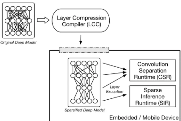
To examine the SparseSep techniques, we prototype three software components: Layer Compression Compiler, Sparse Inference Runtime and Convolution Separation Runtime; these are briefly described below, and shown in Figure 2.
Sparsified Deep Model Sparse Inference Runtime (SIR) Convolution Separation Runtime (CSR)
Embedded / Mobile Device Layer Compression
Compiler (LCC)
Original Deep Model
Layer Execution
Figure 2: SparseSep Framework and Operation
Layer Compression Compiler (LCC).Prior to a deep model being used on a wearable device, it is processed to apply sufficient compression to satisfy device constraints. No machine learning expertise is required, developers only specify constraints of the target hardware to LCC including the memory limits and computational constraints in terms of execution time. LCC automatically applies the sparse coding-based factorizations described above throughout the deep model. The objective is to determine a set of insertion positions and compression degrees that match the required resource constraints, while also minimizing any loss of accu-racy. In§4, this procedure is described in detail as well as how the search for the optimal configuration of compression layers is performed efficiently.
Sparse Inference Runtime (SIR).To maximize the ben-efit of the model produced by LCC, modifications are re-quired to the fully connected layers of DNNs/CNNs. First, compaction layers are k-sparse and it requires a series of key modifications to be made on the standard feed-forward style inference approach across the modified model. The modifi-cation heavily utilizes the inherent sparse structure of the generated weight matrices to gain computational efficiency. Second, to assist those platforms that are constrained by memory severely, layers are executed one by one. For in-stance, only the matrices related to the specific two layers being executed are loaded into the memory and computed on. The decision to do this for a layer pair is taken by the compiler and done conservatively if it is expected to in-troduce unwanted delays in the inference time due to the overhead of additional load times.
Convolution Separation Runtime (CSR). To further minimize the inference time of a CNN model, after modi-fied by the LCC, convolution layer modifications are needed. The time constraint provided by a developer is again used to select a set of convolutional layers and their compression levels are determined to meet the overall resource goals. In the case of severe memory unavailability, strategies similar to SIR are employed (see §4.4). The goal here is to keep the functional behavior of the modified model as close as possible to the original unmodified model.
4. ALGORITHMIC FOUNDATIONS
The core components of SparseSep rely heavily on a number of algorithms to select, compress, and optimize both fully connected and convolution layers of deep models. In the
following we begin by briefly explaining the computational requirements of typical deep models (e.g., DNN and CNN). We then provide intuitions for optimizations, describe in detail the sparse weight factorization and the convolutional separation approaches employed by SparseSep, and highlight the necessary conditions and benefits of the techniques on memory footprint and computational efficiency.
4.1 Deep Model Computations
The inference task of DNNs can be summarized as a series of matrix multiplications, vector additions and evaluations of non-linear functions. For example, the outputoof neural network with a single hidden layer can be computed as:
o= SoftMax b2+W2·f(b1+W1·x) , (1) where x is the input vector, f(·) is the non-liner function (e.g.,sigmoid), bi is the bias vector and Wi is the weight matrix associated with layer i. The matrix operations can be efficiently computed using, e.g., a GPU, while applying new vectorization techniques [21]. Development of computa-tional optimization is complementary to the development of efficient hardware, as it often enables running a deep model more efficiently on the new platform. However, GPUs are seldom available on wearable platforms due to their large en-ergy footprints. We address both memory and computation optimization tasks for fully connected layers by drawing in-spirations from the well-knownmatrix chain multiplication
problem [22].
In case of a CNN with one convolution, one pooling and one hidden layer, the outputocan be computed as:
o= SoftMax b2+W2·maxpool [M] , (2) where, M is thefeature map computed from the 2D input
xas: Mj=f X c xc⇤Kcj+b1j ! , (3)
where,crepresents the index over channels andKis the set of learnable convolution kernels.
4.2 Weight Factorization
In case of a fully connected layer, updating states of all nodes requires evaluating the product:
WL·xL (4)
where, xL2Rn is the state of nodes in the previous layer
and WL
2 Rm⇥n is the matrix representing all the
con-nections between layer L and L+ 1. Now, the basic idea in decreasing the number of required computations is to re-place the weight matrixWLwith a product of two di↵erent
matrices, i.e.,
WL=U·V (5)
where U 2Rm⇥k, V
2Rk⇥n, such that the total number
of computations needed to compute U ·(V ·xL) becomes
smaller than the original multiplication (see Equation 4). In other words, computational efficiency can be achieved, when the total number of multiplications inU·(V ·xL) is smaller
than the number of multiplications inWL
·xL, i.e.: k·n·1 +m·k·1 < m·n·1 (6)
=) k < m·n
W
Lx
Lx
L+1U
V
x
L+1x
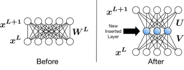
L New Inserted Layer Before AfterFigure 3: Layer insertion to achieve computational efficiency
Hence, the above equation gives us a rule for selecting the di-mensionality ofUandV matrices to achieve computational efficiency. The computational gain due to the factorization of weight matrixWLcan be easily implemented by first
re-moving the connectionsWL, followed by introducing a new
layer withk nodes1 and finally updating new connections to the adjacent layers with weights V and U respectively. Figure 3 illustrates the architectural modifications needed to allow weight factorization-based optimizations.
Weight factorization also brings memory benefits. For exam-ple, before any architectural modifications, the total num-ber of parameters needed to compute xL+1 is m·n+m, i.e., all the elements of matrixWL and the biases of layer L+ 1. Once the weight matrix is factorized and replaced,
n·k+k·m+mparameters are required for evaluatingxL+1. Interestingly, a decrease in model size can be achieved if the following inequality holds:
n·k+k·m+m < m·n+m, (8) The above inequality simplifies to the same requirement as identified in Equation 7. The space gain Sg due to layer
modification can be defined as:
Sg= m·n+m
n·k+k·m+m (9)
Ideally, we seek a factorization resulting inSg 1.
4.3 Weight Reconstruction
Note that, under loss-less factorization, i.e., no error in the reconstruction ofWL, the modified architecture of the deep
model stays functionally equivalent to the original. However, often arbitrary factorizations of large matrices introduce re-construction errors and thus the new constructed model de-viates from the original model and a↵ects the oveall per-formance accuracy. Thus, care should be taken to keep the reconstruction error (e.g.,L2-norm) as small as possible, i.e.:
||WL U·V||22⇡0 (10)
Previously, optimization of DNN models have been attempted using the well establishedSingular Value Decomposition(SVD) approach [23, 24]. Under SVD, the weight matrix can be ef-ficiently factorized as:
WmL⇥n=Xm⇥m·⌃m⇥n·NnT⇥n, (11)
where, ⌃m⇥n is a rectangular diagonal matrix containing singular valuesofWL
m⇥nas the diagonal elements. To gain
1We also set the bias of each node to 0 and no no-linearity
function is added.
computational efficiency the weight matrix can be approxi-mated well by keepingk highest singular values, i.e.:
Wm⇥nL ⇡Xm⇥k·⌃k⇥k·Nk⇥nT (12)
Now, the architecture of a fully connected layer of a deep model can be modified by replacingWL withU =Xm
⇥k
andV =⌃k⇥k·NkT⇥n (see Figure 3).
4.4 Sparse Coding-based Factorization
In the following, we propose a novel technique of improving the memory and computational gains over the SVD-based factorizations (for a givenk). These gains are essential for efficiently running deep models on low-end wearables. The sparsity requirement also makes SparseSep novel from our previously published DeepX system [14].
4.4.1 Dictionary Learning
The basic idea is to come up with a sparse factorization of the weight matrixWL. In other words, if either of theU or V matrices can be made sparse, further space savings can be achieved. Furthermore, sparse matrix multiplication also helps to improve overall computational time. In this work, we introduce the use of sparse coding-based factorization technique of fully connected layer weights to achieve very low memory and computational footprint.
The sparse matrix factorization problem can be formulated as a sparse dictionary learning problem, where a dictionary
B = { }k
i=1 (with i 2 Rm) is learned from the weights WLof a fully connected layer of a deep model using an
un-supervised algorithm. Sparse coding approximates an input
wi2 Rm, e.g., a column of WL, as a sparse linear
combi-nation of basis vectors from the dictionaryB[25, 26, 27], i.e.: wi= k X j=1 aij· j, (13)
where,aiis a sparse vector, i.e., majority of its elements are 0. A large number of dictionary learning algorithms have been proposed in the literature and in this paper we use the K-SVD algorithm [28] to learn a dictionary comprising ofk
basis vectors. The K-SVD algorithm learns a dictionary by solving the following minimization problem:
min B,A||W
L
B·A||2
2 s.t.8i||ai||0K (14)
where A 2 Rk⇥n is the sparse code of the weight matrix WLunder the dictionaryB
2Rm⇥k andK is the sparsity
constraint factor, i.e., each signal is reconstructed with fewer thanKbasis vectors. Once the dictionaryBand the sparse codeAis learned, we obtain the sparse factorization ofWL
as:
WL⇡B·A (15)
4.4.2 Architecture Modification
To gain computational and space efficiency, we interpose a new layer similarly as described in§4.2, while settingU =B and V = A (see Figure 3). DNN and CNN models of-ten have more than one fully connected layers and thus the sparse factorization technique can be applied on all of these layers to improve overall inference efficiency.
4.4.3 Quality of Code Book and Sparsity
The success of the sparse factorization of weights depends on the quality of the learned dictionary, its reconstruction quality and the sparsity of the generated code. However, as in the case with the SVD approach, the dictionary learning with sparsity constraint introduces reconstruction error and the modified model deviates from the original model in the parameter space. Deviation in the parameter space often adversely a↵ect the performance quality of the model and thus care should be take to maintain the reconstruction er-ror at low as possible. This can be achieved by introducing a hyper parameter↵[27] that assigns a greater importance in minimizing the reconstruction error term than the sparsity requirement as given in Equation 14. In computer vision and audio recognition tasks, often over-complete dictionar-ies are learned for resilient feature learning. However, in line with our objective of achieving space and computational ef-ficiency, we extract a compact representation of deep model parameters by learning a small dictionary.
4.4.4 Memory Gain
One of the main advantages of making sparse factorization of fully connected layers, over techniques using SVD, is its ability to reduce memory footprint significantly. For exam-ple, the space gain under sparse factorization becomes:
Sg⇤=
m·n+m
2⇤nnz(A) +k·m+m, (16)
where,nnz(A) counts the number of non-zero elements in matrix A. The factor 2 is used to take into account stor-age for indices2 of the non-zero elements of a sparse
ma-trix. Thus, sparse factorization outperforms SVD in terms of memory by a factor of:
Sg⇤ Sg = n·k+k·m+m 2⇤nnz(A) +k·m+m (17) = 1 + n·k 2⇤nnz(A) 2⇤nnz(A) +k·m+m (18) Thus, for nnz(A) < n·k/2, S⇤ g > Sg. Hence, we get a
rule for selecting the variableK in Equation 14 suitably to reduce the bottle neck in memory.
4.4.5 Execution Pipeline
The main purpose of LCC is to bring sparse factorization as an o✏ine tool for modifying large deep models. The feed-forward architecture of DNN allows a unique opportunity to apply a layer-wise partial inference scheme. Under this approach, layers of a DNN are sequentially loaded in the memory and their output is retained. Given the maximum memory, we can estimate the number of nodesk to use in the inserted layer for a pre-defined sparsity amount, e.g., 15%. In extreme cases, when two matrices can not simulta-neously be loaded on the memory, simple tricks like divide and conquer approach to matrix multiplication can be em-ployed that only require partial portions of the matrices in the memory. Partial multiplication of matrices, however, in-creases paging amount, which inin-creases the overall inference time.
Contrary to the constraint on available memory, satisfying a given limit on the accuracy degradation is non-trivial.
2In case of contiguous memory allocation, one index is
enough to identify elements in a matrix.
Algorithm 1Satisfy Accuracy Constraint
1: Input:(i)M: a DNN/CNN, (ii)V: a validation dataset and (iii) AT H: max allowed degradation in accuracy
(e.g., 5%)
2: Output: (i) ˆM: an optimized DNN/CNN 3: FCLayer := findAllFCLayers(M)
4: fori:= 1 :length(FCLayer)do
5: ku:=getU pperBound(F CLayer[i].W) .Getting
an estimate fork using Equation 7 6: kl:= 1
7: kc:=kl
8: whileTruedo .Searching for suitablek in the range (kl, ku) using binary search
9: kc:=updateBinarySerchParameter(kc, kl, ku)
10: U,V :=sparseF actorize(F CLayer[i].W, kc)
11: newLayer:=constructN ewLayer(U,V) 12: Mˆ :=replaceLayer(F CLayer[i], newLayer) 13: DA:=getP erf ormanceDeviation( ˆM,V)
14: if DA< AT H then
15: SaveModel( ˆM)
16: Break
17: ReturnreadSavedModel()
This is because of the fact that there is no linear correla-tion between the reconstruccorrela-tion error and the model accu-racy. Little variations in the weights can force a number of nodes to switch states, thereby potentially a↵ecting the inference quality. To mitigate the problem we rely on a val-idation dataset provided along with the model and employ a search strategy to satisfy the accuracy degradation limit. Algorithm 1 provides an overview of the search procedure. Given the model, validation dataset and accuracy degrada-tion bound, the algorithm searches for sparse factorizadegrada-tion of one or more fully connected layers. For each layer, the algorithm follows a binary search procedure to estimate a suitable value fork and measures the accuracy degradation after applying sparse factorization of the weight matrix and replacing the layer as shown in Figure 3. If the accuracy bound is satisfied, this sparse factorization is accepted and the algorithm proceeds to the next fully connected layer. Inference time of a DNN model, among other things, pri-marily depends on its parameter size and on the processing capabilities of the hardware. We take opportunistic advan-tage of Algorithm 1 and log all values ofkused in individual layers (i.e., independent variables) and inference time (de-pendent variable) to build a simple regression model. The regression model can predict the execution time given para-metric setting of k values in each layers. If the time pre-diction is higher than the given time constraint, we neglect saving the model. For example a simple conditional state-ment on time after line–14 in Algorithm 1 can be added to satisfy the time constraint.
4.5 Convolution Kernel Separation
In addition to the large memory requirement, the other bottleneck common in CNN-based inferencing (contrary to DNNs) is the massive amount of convolution operations. Weight factorization does not help to overcome this bottle-neck. In the following we summarize techniques to mitigate this challenge.
4.5.1 Convolution Complexity
The time complexity of convolving a single channel 2D-input (H⇥W) with a bank ofN d⇥dfilters isO(N d2HW). For large input image stacks withC channels, the runtime can be significantly large [29], e.g.,O(CN d2HW). One way to
reduce the time complexity is by reducing the redundancy among di↵erent filters and filter channels [30]. Although, ap-proximation techniques using linear combination of a smaller set of filters have been successfully attempted [29], in this work we exploit separable filter property to reduce the over-all convolution operations.
4.5.2 Separable Filters
LetK2RN⇥d⇥d⇥Cbe the set of convolutional kernels (4D),
here the goal is to find an approximation ˆK, which can be decomposed as [31]: ˆ Kcn= K X k=1 Hkn(Vkc)T, (19)
where, the parameterKcontrols the rank of thehorizontal filterH2RN⇥1⇥d⇥K and thevertical filter
V2RK⇥d⇥1⇥C.
Under this approximation scheme, the original convolution task of a single 3Dfilter3(indexed byn) becomes:
Kn⇤x ⇡ Kˆn⇤x = C X c=1 K X k=1 Hk n(Vkc)T⇤xc = K X k=1 Hkn⇤ C X c=1 Vkc⇤xc ! (20)
4.5.3 Architecture Modification
BothH and V filters can be learned from the pre-trained filterK. In this work we adopt a deterministic SVD-based approximation algorithm, as given in [31], to estimateH,V. Interestingly, Equation 20 shows that the overall convolu-tion task can be broken down into two sets of convoluconvolu-tions. First, the inputxis convoluted with the vertical filterVto produce an intermediate feature map Z. Next, Z is con-voluted with the horizontal filterHto generate the desired output. Thus, the original convolution layer of the CNN now can be replaced with two successive convolution layers with filtersVandHrespectively.
4.5.4 Computational Gain
Under this separation, the overall time complexity becomes
O(CKdHW +KN dHW) orO(dK(N+C)HW). Now for computational efficiency, the parameterKshould be chosen such that:
K < dCN
C+N (21)
As described in §4.3, for keeping the functionality of the modified model as close as the original model, the recon-struction error of the convolution filter should be very low, i.e.,
||K K||ˆ 2
2⇡0 (22)
3The 4D filter bank
Kcan be viewed as a collection of N
3Dfilters.
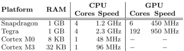
Platform RAM CPU GPU
Cores Speed Cores Speed
Snapdragon 1 GB 4 1.2 GHz 6 450 MHz Tegra 1 GB 4 2.3 GHz 192 950 MHz Cortex M0 8 KB 1 48 MHz
Cortex M3 32 KB 1 96 MHz
Table 1: Summary of the Hardware Platforms
4.5.5 Runtime Adaptation
As part of SparseSep, we developed a runtime framework that dynamically selects convolution layers and their sepa-ration criteria to adapt the overall computations needed for a CNN according to the current availability of computation resources or constraints. The runtime adaptation approach follows very closely the binary search procedure outlined in Algorithm 1. Instead of the fully connected layers, the algo-rithm begins by constructing a list of available convolution layers. An upper bound of the filter separation parameter
K is estimated using Equation 21. Hand V filters are es-timated for the selected separation parameter K as given in [31]. Next, the current convolution layer is now replaced with two successive convolution layers with filtersVandH and the updated model performance is computed on the val-idation dataset. If the error criterion is satisfied, the modi-fication is accepted and the procedure moves on to the next convolution layer.
Runtime convolution operation optimization opens up new opportunities for SparseSep to gracefully shape and control resource consumption of both DNNs and CNNs on a large variety of hardware platforms, which is not possible for sys-tems like DeepX [14].
5. EVALUATION
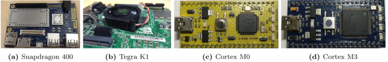
In this section we systematically summarize results from a number of experiments to highlight the main benefits of the sparse weight factorization and convolution separation tech-niques presented above. As the target wearable hardware we consider four platforms: (i) Qualcomm Snapdragon 400 SoCs, (ii) Nvidia Tegra K1, (iii) ARM Cortex M0 and (iv) ARM Cortex M3. Hardware specifications for the four plat-forms are summarized in Table 1.
5.1 Experimental Setup
In this paper we focus on audio inference as the represen-tative wearable and mobile sensing tasks to infer the sit-uational context of users’ surroundings. We train and de-ploy DNN models to recognize the ambient environment of the user and to identify the speaker from voice recordings. We apply our factorization technique to CNN models by considering two state-of-the-art object recognition models: AlexNet and VGG. However, do could not run the CNN models on the ARM Cortex platforms for severe memory limitations (allowing only 8 KB and 32 KB).
5.1.1 Audio Datasets
We consider two large publicly available audio datasets: (i) LITIS Rouen Audio scene dataset [32] and (ii) Automatic Speaker Verification Spoofing and Countermeasures Chal-lenge Dataset [33].
The Audio Scene dataset, referred in this paper as the Am-bient dataset, contains over 1500 minutes of audio scenes,
(a)Snapdragon 400 (b)Tegra K1 (c)Cortex M0 (d)Cortex M3
Figure 4: Hardware platforms: (a) Qualcomm Snapdragon 400 and (b) Nvidia Tegra K1 are used to evaluate the proposed scaling benefits of weight factorization and convolution separation techniques. Additionally, we use (c) ARM Cortex M0 and (d) M3 to evaluate DNN performances.
which were captured using Samsung Galaxy S3 smartphones. The dataset is composed of 19 di↵erent ambient scenes such as, ‘plane’, ‘busy street’, ‘bus’, ‘cafe’, ‘student hall’ and ‘restaurant’. Audio measurements were recorded with a sampling frequency of 22.05 KHz and several 30 seconds long audio files from each ambient environment are made available.
The Audio Speaker Verification dataset, referred in this pa-per as the Speaker dataset, contains speech recordings from 106 individuals (45 male and 61 female). In addition to the clean voice recordings, the dataset also contains synthesized data for conducting spoofing attacks, however, in this paper we only focus on clean audio recordings from all 106 par-ticipants. Audio measurements were recorded with 16 KHz sampling frequency. To maintain a near equal class distribu-tion, we restrict the maximum duration of audio recording to 15 minutes per user.
For the CNN models, we dowloaded pre-trained models from the ca↵e zoo repository and we use the original test dataset to measure the overall recognition performances of these models. In Table 2 we summarize all deep models studied in this work.
5.1.2 Deep Architecture Training
Small neural networks, e.g., models with a single hidden layer, can be efficiently trained using the well known back-propagation algorithm [34]. However, deep architectures, es-pecially with many hidden layers, are difficult to train and development of efficient training algorithms are an active area of research in machine learning. Past years have seen the development of unsupervised pre-training approaches for better intialization of the layer weights. In this work we use denoising autoencoders to pre-train the weights of the deep architecture and apply the back-propagation algorithm to fine tune architecture for classification purposes. Before training the audio models, we follow a sliding window ap-proach, as described in [32], to extract 13mel-frequency cep-stral coefficients(MFCC) from a measurement window of 25 milli seconds. The extracted MFCC features are then aggre-gated over a 5 second period to generate an input feature dimension of 650, see [32] for details. For both the dataset we follow the same data pre-processing approach. Finally, we train DNN models with two hidden layers (each having 1,000 nodes) on both datasets and use early stopping crite-ria to avoid over-fitting.
5.1.3 Hardware
We evaluate the performances of the weight factorization and convolution separation techniques, while executing DNNs and CNNs, on Qualcomm Snapdragon 400 [35] and Nvidia Tegra [15]. To highlight the benefits of sparse factorization,
Name Type Parameters Architecture
AlexNet CNN 60.9M c:5ı;p:3‡;fc:3?
VGG CNN 138.4M c:13ı;p:5‡;fc:3?
Ambient DNN 1.7M fc:3?
Speaker DNN 1.8M fc:3?
ı
convolution layers;‡pooling layers;?fully connected layers
Table 2: Representative Deep Models
we also perform experiments by running the DNN models on ARM Cortex M0 and M3.
The Snapdragon 400 SoC [35] is widely available in many smartwaches, e.g., LG G smartwatch R [36]. Figure 4a shows a snapshot of the Snapdragon development board used in our evaluations. Primarily designed for phones and tablets, it contains 3 processors: a Krait 4-core 1.2 GHz CPU, an Adreno 306 GPU and a 680 MHz Hexagon DSP. We find the CPU can address 1GB of RAM, but the DSP only 8MB. All our experiments on Snapdragon were conducted using its CPU only.
Although, not as popular as the Snapdragon, the Tegra K1 [15] (Figure 4b) provides extreme GPU performance, un-seen in other mobile SoCs. The heart of this chip is the Ke-pler 192-core GPU, which is coupled with a 2.3 GHz 4-core Cortex CPU and an extra low-power 5th core (LPC). The K1 SoC is used in the Nexus 9, Google’s phone prototype within Project Ara [37], and even high-end cars [38]. It is also used in IoT devices like the June Oven [39]. Executing code on the LPC requires the toggling of linux system calls, while access to the GPU is available from CUDA drivers [40]. The ARM Cortex-M series are examples of ultra-low power wearable platforms. The smallest of them all is Cortex M0, which consumes 12.5µW/MHz and support a memory size of 8 KB (Figure 4c). The M3 variant (Figure 4d) of the cor-tex has double processing abilities (96 MHz) and support a 32 KB memory. These low-end micro-controllers often have limited memory management capabilities. In our experi-ments we could only use around 5.2 KB memory on Cortex M0 and around 28 KB memory on Cortex M3. Availability of a small memory requires frequent paging, while executing a large model. The I/O capabilities of Cortex M0 was found to be significantly slower than Cortex M3. For prototyping, we use MBED LPC11U24 [41] and LPC1768 [42] boards for running experiments on Cortex M0 and M3 respectively.
5.2 Scalability Under Sparse Factorization
Next, we study the accuracy of modified DNN model and its space requirements under factorization of fully connected layer weights. Although, the principle of weight factoriza-tion can be simultaneously applied to all fully connected
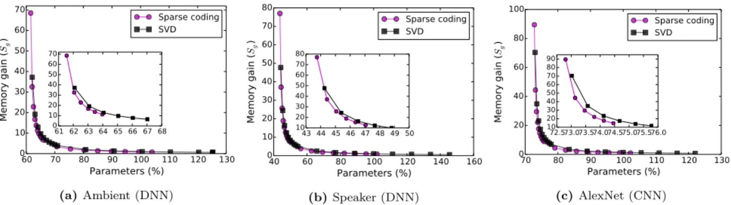
(a)Ambient (DNN) (b)Speaker (DNN) (c)AlexNet (CNN)
Figure 5:Comparison of memory gains with reduced hidden layer nodes when using sparse coding- and SVD-based weight factorizations for DNNs and CNNs. For simplicity of illustrations, factorization of one fully connected layer of all three models are considered. For all the models, sparse factorization generated much smaller model compared to the SVD-based factorization.
(a)Ambient (DNN) (b)Speaker (DNN) (c)AlexNet (CNN)
Figure 6:Comparisons of recognition accuracy performances with reduced hidden layer nodes when using sparse coding- and SVD-based weight factorizations for DNNs and CNNs. In our experiments we allow a maximum of 5% degradation in accuracy from the original model performance. Sparse factorization maintains high accuracy, similar to SVD approach, but generates models with smaller memory footprint. Similarly as above, we factorize only one layer.
layers of a DNN, for simplicity of understanding, we only focus on one layer of the DNN and study the e↵ect of the factorization.
Figure 5 illustrates the space or memory gain that can be achieved over the original models (two DNNs and one CNN) under sparse and SVD-based factorizations for various sizes of the new inserted hidden layer. Note that, the high range in Y-axis in both the figures indicate that the sparse coding-based approach provides a significantly better scalability over the SVD solution (see the insets). For example, the smaller the number of nodes kept in the inserted hidden layer, higher is the gain in memory. Additionally, the gain also comes from the sparse matrix multiplications and in this experiment we keep the sparsity level at 20%, while perform-ing the dictionary-based weight factorization. Sparse codperform-ing is seen to consistently maintain a superior gain over SVD. Figure 5 also indicates that a larger value of nodes in the inserted hidden layer can adversely increase the space re-quirement of the model, thus making it inefficient. Finally, the criterion for selecting a good value for k, as given in Equation 7, can also be empirically understood from the figures. SVD looses memory gain when k retains around 80% of the hidden layer parameters. For a layer with 1,000 nodes, ak value of 80% will results in less than 400 nodes in the inserted new layer. From Equation 7 we empirically findk= m·n
m+n =
650⇤1000
650+1000 ⇡394, thus verifying the
mathe-Figure 7: Memory requirements of four original deep learning models studied in the paper. Ambient and Speaker are two audio-based DNN models, whereas AgeNet and AlexNet are two image-based CNN models.
matical intuition given earlier.
Seeing sparse factorization giving rise to a great memory benefits, we next study the e↵ect of factorization on model performance. Figure 6 illustrates the accuracy performance of the models (same two DNNs and one CNN as given in Figure 5) under both types of weight factorizations. As in-dicated before, under faithful factorization of the model, i.e.,
WL=U·V, the modified model would have the same func-tional properties, i.e., same accuracy. However, as we search for smallkthe reconstructions starts to deviate significantly fromWLand the model accuracy is observed to violate the
(a) Ambient (DNN) (b)Speaker (DNN)
(c)AlexNet (CNN) (d)VGG (CNN)
Figure 8: Energy-consumption and average inference time of di↵erent variants of the deep models on four di↵erent hardware platforms.
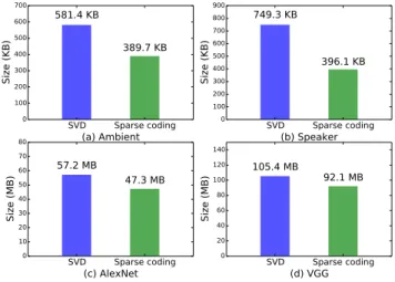
Figure 9: Memory requirements of the four deep models under SVD- and sparse weight factorizations
accepted (pre-defined) 5% tolerance level. Interestingly, for majority of the chosen values ofk, both sparse coding and SVD exhibit accuracy very close to the original DNN. Thus, the factorization approach can reduce memory footprint sig-nificantly, while maintaining high accuracies.
Figure 7 illustrates the original (uncompressed) model sizes for all the four DNN/CNN models considered in this work.
The two DNN models are much smaller in size and depth, compared to the CNN models. However, after our factoriza-tions the memory footprints of the models are highlighted in Figure 9. To obtain an optimized model we execute Al-gorithm 1 with the models and allow an accuracy toler-ance level of 5%, the algorithm performs factorization on all fully connected layers of the model and generates a com-pact version of the model. This figure indicates the ability of the Sparse factorization to achieve significantly smaller and equal functional models as provided by the SVD technique. The memory is one of the main bottlenecks in low end plat-forms such as Cortex M series, and thus Sparse coding tech-nique allows for a better tradeo↵solutions by significantly reducing the amount of required paging.
Although, we focussed mainly on the factorizations of DNN layer weights, the basic idea applies to a subset of layers within CNN models. For example, in addition to the con-volution and pooling layers, often a CNN has one or more fully connected layers, e.g., for classification purposes. These fully connected layers are ideal for sparse factorizations to gain computational and memory efficiencies. Thus, as the final set of experiments we apply our proposed sparse factor-ization on the AlexNet model, which is a popular computer vision (CNN) model trained for recognizing objects within natural images. However, later we show that the main com-putational benefits of CNN models arise mainly from the separation of kernel approach.
Contrary to the model used for Ambient or Speaker iden-tification, the original AlexNet model is much larger, e.g., contains 61 million parameters [12], and requires a storage space of 233 MB. When applied sparse factorization to its first fully connected layer only, memory requirement reduces from 233 MB to below 100 MB. Figure 5c and 6c respectively shows memory gain and accuracy deviations for various sizes of the inserted hidden layer.
5.3 Runtime and Energy Performances
We now turn our attention to evaluating runtime and en-ergy performances of sparsely factorized DNNs and CNNs on the four wearable hardware platforms (Cortex M series are only used to evaluate DNNs). For the CNN models we also evaluate the performance of the convolution separation approach on runtime and energy consumption.
To measure runtime and energy performances, we next run the original, the factorized models, and the convolution sep-arated models (incase of CNNs) on the four hardware plat-forms. The results of the experiment are presented as a tradeo↵ study in Figure 8 for all four individual models. Not only space scalability, the reduced number of param-eters significantly improves the running time of the sparse model on all platforms (note the log scale on both the axes). For both the ambient and speaker models (DNNs), the av-erage4inference time is observed to vary significantly across platforms. However, the e↵ects of factorizations of DNNs are significant on all platforms. Overall, the sparse factor-ization generating better running time over SVD. On both Snapdragon and Tegra, the factorized DNNs runs under one milli second, resulting in around 5 times faster infer-ence than the unmodified model. Similarly to the running time, sparse factorization helps to drop the average energy consumptions significantly on all platforms. For example, on Cortex M0, the power consumption becomes one tength. On Snapdragon 400, the optimized DNN model now consumes only 56% of energy compared to the unmodified model. Most interesting performance gains are observed for the CNN models, while applying the convolution separation (CSR) technique in conjunction with the weight factorization (LCC). On both Snapdragon and Tegra, the VGG model is seen to be benefitted the most, as it contains significantly high (13) numbers of convolutional layers than AlexNet (see Table 2). The overall running time of the optimized VGG model is just over 1.5 sec on Snapdragon, which is around 2.7 times faster (little below the theoretical upper limit of 3) than its sparse weight factorized only variant.
Thus the techniques presented in the paper open up new op-portunities to drastically reduce the memory footprint and overall computational demands of state-of-the-art deep mod-els. We believe that our work will make deep learning based inference engine on wearable and IoT devices highly popular and will help to redefine mobile and IoT experiences.
6. DISCUSSION
We briefly examine a range of key issues related to Spars-eSep, along with the limitations of our approach.
Broader Deep Learning Support. Our approach has been tested on the two most popular forms of deep learning –
4All inferences are repeated 1,000 times and we report their
averages in the figures.
DNNs and CNNs – which both include fully-connected feed-forward layers. Any deep model that includes this layer type will benefit from sparse weight factorization of SparseSep. Moreover, the convolution separation technique of Spars-eSep will allow further optimization of CNNs. Although the mixture of layer types within a model will influence the gains, for example, CNNs have more convolutional layers than feed-forward layers, thus are benefited the most from SparseSep; however, feed-forward layers in CNNs account typically for 80 to 90% of all the memory consumed [12, 20] making them an important target for memory-centric optimizations. Extending the ideas of SparseSep to other forms of deep learning, such as RNNs and LSTMs, remain as important future work.
Hardware Portability. To keep the usage of SparseSep simple for developers we allow them to express constraints to LCC in terms of accuracy, memory and execution time. However, supporting execution time requires SparseSep to estimate the performance of a specific deep model archi-tecture (i.e., layers and node configuration) on the target hardware. SparseSep includes only a fairly simple estima-tion process based on data from hardware profile process. In our experiments, profiling hardware takes only around 30 minutes using an automated script that tests various model architectures while the device is attached to a power moni-tor.
Hardware Accelerators. Purpose-built hardware accel-erators for deep learning are beginning to emerge [43, 6]. While none of them are currently suitable for wearables yet; more importantly, SparseSep will remain useful even when accelerators become available due to the substantial savings in resource usage o↵ered with only a minimal impact on ac-curacy. This will allow accelerators to execute even larger models than currently possible. Moreover, the reductions in resources enabled by SparseSep will facilitate the design of more energy efficient deep learning accelerators, better suited to wearables than today, because they can be built with fewer computational and memory resources than pre-viously possible.
7. RELATED WORK
We now overview work closely related to SparseSep, this in-cludes results from the compressive sensing area, and e↵orts to lower resources used by sensing algorithms.
Optimizing Mobile Sensing Algorithms. The chal-lenge to mobile resources of executing the algorithms neces-sary to extract context and user activities from sensor data has been long recognized and studied. Approaches include the development of sensing algorithm optimizations such as short-circuiting sequences of processing or identifying effi -cient sampling rates and duty cycles for sensors and algo-rithm components like [44, 45, 46]. Work such as [47] aims to combine such optimizations along with careful usage of energy efficient hardware. Others [48] take a stream view and so applies stream oriented optimizations on the basis of real dataflows arriving from sensors. [49] approaches perfor-mance tuning by extending ideas of feature and model selec-tion to consider device resources, and even cloud o✏oading opportunities.
In sum, SparseSep is the most recent of this chain of work, but di↵ers importantly in the fact that it is one of the few
to investigate deep learning specific methods exclusively – this in turn allows SparseSep to highlight significant oppor-tunities for gains (such as memory and computation) that only exist within such models. It is likely that many of the other techniques described could operate in combina-tion with SparseSep given they frequently treat the learning algorithm itself as a black-box. However, they may bring un-desirable negative side-e↵ects such as higher levels of accu-racy loss. More broadly, one could characterize the de-facto approach to using deep learning in wearables and mobile devices today as being based on cloud-based, and therefore approaches like MAUI [50] and those related to it are appli-cable. However, such approaches su↵er from problems in-cluding challenges to privacy protection when partitioning deep models as highlighted in§1.
Deep Learning under Resource Constraints. Ex-amples of deep models designed specifically for wearable constraints are still maturing. A popular approach is for experts to hand optimize specific deep models targeting a specific device class (e.g., smartphone). This has been done for machine translation [10], speaker identification [51] and keyword spotting [11] (i.e., a device constantly waiting for a small number of specific phrases). Moderately-sized DNNs designed specifically for constrained processors (like the DSP) in smartphones have also be demonstrated [8, 52] for a range of audio sensing tasks, as well as basic activity recognition scenarios. Discussions of the techniques used to optimize these models are slowly now being reported [20]. In contrast, SparseSep enablesautomatedoptimization broadly applica-ble to deep model families (DNN and CNN). There is little cost for SparseSep to be applied to new/revised models, or when resources change (e.g., a new device is released). Naturally, work is also increasing in the area of more system-atic easily re-used techniques for lowering resource consump-tion in deep models. A common framework for these ap-proaches is from the machine learning community and called
model compression that most often used at training time (unlike SparseSep that is inference-time focused) to scale to larger datasets or increase hardware utilization. Tech-niques of this type vary in particular to the extent to which the underlying model is altered. For example, [24] actually removes nodes and reshapes layers within the model while [21, 53] performs types of quantization of parameters within layers. We design SparseSep towards minimizing the mod-ifications made to the model and so adopt approaches that
insert new layers designed to optimize performance. SVD-based methods of this type are the current state of the art (such as [54]) which SparseSep has numerous advantages as detailed throughout this paper. [14] focuses on how to parti-tion deep learning models across di↵erent types of processors (GPUs, CPUs, DSPs) found within an system-on-a-chip; it uses an SVD-based model compression approach to allow a partition of a model to fit within the resources of a specific processor (such as a DSP). SparseSep in contrast is agnos-tic to processor type, and complementary to [14] in that its performance could only improve if it incorporated ideas of utilizing a spectrum of processors.
8. CONCLUSION
In this paper, we have proposed SparseSep – a set of novel techniques for optimizing large-scale deep learning models – that allows deep models to function even under the extreme
system constraints presented by wearable hardware. Con-ceptually, SparseSep brings many of the recent advances in sparse dictionary learning and convolution kernel separation to how deep learning models are both represented and exe-cuted. The core innovation is an o↵-line method to sparsify the internal feed-forward layers of both DNNs and CNNs, and optimization of convolution filters of CNNs, that pro-duces a highly compact model representation with only small reductions in classification accuracy. Such layer sparsity in turn, enables SparseSep to re-invent the inference process used in deep models and allow classification to occur with radically lower resources. We believe the leaps in deep learn-ing inference efficiency that SparseSep provides will prove to be a significant enabler for the broader adoption of such modeling techniques within mobile and IoT platforms.
9. ACKNOWLEDGEMENTS
We would like to thank our Shepherd, Prof. Bhaskar Krish-namachari, for his valuable comments and time to improve the overall quality of this paper. We also thank Ray Kear-ney from Nokia Bell labs, Dublin for helping us in building the power monitoring tool for ARM Cortex boards.
10. REFERENCES
[1] Y. Bengio, I. J. Goodfellow, and A. Courville, “Deep learning,” 2015, book in preparation for MIT Press. [Online]. Available:
http://www.iro.umontreal.ca/˜bengioy/dlbook [2] L. Deng and D. Yu, “Deep learning: Methods and
applications,” Tech. Rep. MSR-TR-2014-21, January 2014. [Online]. Available:
http://research.microsoft.com/apps/pubs/ default.aspx?id=209355
[3] G. Hinton, L. Deng, D. Yu, G. Dahl, A. rahman Mohamed, N. Jaitly, A. Senior, V. Vanhoucke, P. Nguyen, T. Sainath, and B. Kingsbury, “Deep neural networks for acoustic modeling in speech recognition,”Signal Processing Magazine, 2012. [4] Y. Taigman, M. Yang, M. Ranzato, and L. Wolf,
“Deepface: Closing the gap to human-level performance in face verification,” inConference on Computer Vision and Pattern Recognition (CVPR), 2014.
[5] K. J. Geras, A. Mohamed, R. Caruana, G. Urban, S. Wang, ¨O. Aslan, M. Philipose, M. Richardson, and C. A. Sutton, “Compressing lstms into cnns,”CoRR, vol. abs/1511.06433, 2015. [Online]. Available: http://arxiv.org/abs/1511.06433
[6] T. Chen, Z. Du, N. Sun, J. Wang, C. Wu, Y. Chen, and O. Temam, “Diannao: A small-footprint high-throughput accelerator for ubiquitous machine-learning,” inProceedings of the 19th
International Conference on Architectural Support for Programming Languages and Operating Systems, ser. ASPLOS ’14. New York, NY, USA: ACM, 2014, pp. 269–284. [Online]. Available:
http://doi.acm.org/10.1145/2541940.2541967 [7] N. Hammerla, J. Fisher, P. Andras, L. Rochester,
R. Walker, and T. Pl¨otz, “Pd disease state assessment in naturalistic environments using deep learning,” in
[8] N. D. Lane and P. Georgiev, “Can deep learning revolutionize mobile sensing?” inProceedings of the 16th International Workshop on Mobile Computing Systems and Applications, ser. HotMobile ’15. New York, NY, USA: ACM, 2015, pp. 117–122. [Online]. Available:
http://doi.acm.org/10.1145/2699343.2699349 [9] “Your Samsung SmartTV Is Spying on You,
Basically,” http:
//www.thedailybeast. com/articles/2015/02/05/your-samsung-smarttv-is-spying-on-you-basically.html. [10] “How Google Translate squeezes deep learning onto a
phone,” http://googleresearch.blogspot.co.uk/2015/ 07/how-google-translate-squeezes-deep.html.
[11] G. Chen, C. Parada, and G. Heigold, “Small-footprint keyword spotting using deep neural networks,” in
IEEE International Conference on Acoustics, Speech, and Signal Processing, ser. ICASSP’14, 2014.
[12] N. D. Lane, S. Bhattacharya, P. Georgiev, C. Forlivesi, and F. Kawsar, “An early resource characterization of deep learning on wearables, smartphones and
internet-of-things devices,” inProceedings of the 2015 International Workshop on Internet of Things Towards Applications, ser. IoT-App ’15. New York, NY, USA: ACM, 2015, pp. 7–12. [Online]. Available:
http://doi.acm.org/10.1145/2820975.2820980 [13] J. Dean, G. Corrado, R. Monga, K. Chen, M. Devin,
M. Mao, M. aurelio Ranzato, A. Senior, P. Tucker, K. Yang, Q. V. Le, and A. Y. Ng, “Large scale distributed deep networks,” inAdvances in Neural Information Processing Systems (NIPS). Curran Associates, Inc., 2012, pp. 1223–1231.
[14] N. D. Lane, S. Bhattacharya, C. Forlivesi, P. Georgiev, L. Jiao, L. Qendro, , and F. Kawsar, “Deepx: A software accelerator for low-power deep
learning inference on mobile devices,” inIPSN 2016. [15] “Nvidia Tegra K1,” http:
//www.nvidia.com/object/tegra-k1-processor.html. [16] “Arm Cortex-M3,” http://www.arm.com/products/
processors/cortex-m/cortex-m3.php.
[17] B. A. Olshausen and D. J. Field, “Sparse coding with an overcomplete basis set: A strategy employed by v1?”Vision research, vol. 37, no. 23, pp. 3311–3325, 1997.
[18] Principal component analysis. Wiley Online Library, 2002.
[19] C. M. Bishop,Pattern Recognition and Machine Learning. Springer, 2007.
[20] A. Krizhevsky, “One weird trick for parallelizing convolutional neural networks,”CoRR, vol. abs/1404.5997, 2014. [Online]. Available: http://arxiv.org/abs/1404.5997
[21] J. S. Ren and L. Xu, “On vectorization of deep convolutional neural networks for vision tasks,” in
Twenty-Ninth AAAI Conference on Artificial Intelligence, 2015.
[22] T. H. Cormen, C. E. Leiserson, R. L. Rivest, and C. Stein,Introduction to algorithms, 3rd ed. MIT press, 2009.
[23] J. Xue, J. Li, and Y. Gong, “Restructuring of deep neural network acoustic models with singular value decomposition,” inINTERSPEECH, 2013, pp.
2365–2369.
[24] T. He, Y. Fan, Y. Qian, T. Tan, and K. Yu,
“Reshaping deep neural network for fast decoding by node-pruning,” inAcoustics, Speech and Signal Processing (ICASSP), 2014 IEEE International Conference on. IEEE, 2014, pp. 245–249.
[25] H. Lee, A. Battle, R. Raina, and A. Y. Ng, “Efficient sparse coding algorithms,” inNeural Information Processing Systems (NIPS), 2007.
[26] R. Raina, A. Battle, H. Lee, B. Packer, and A. Y. Ng, “Self-taught learning: Transfer learning from
unlabeled data,” inProceeding of the International Conference on Machine Learning (ICML), 2007. [27] S. Bhattacharya, P. Nurmi, N. Hammerla, and
T. Pl¨otz, “Using unlabeled data in a sparse-coding framework for human activity recognition,”Pervasive and Mobile Computing, May 2014.
[28] M. Aharon, M. Elad, and A. Bruckstein, “K-svd: An algorithm for designing overcomplete dictionaries for sparse representation,”IEEE Transactions on Signal Processing, vol. 54, no. 11, pp. 4311–4322, 2006. [29] R. Rigamonti, A. Sironi, V. Lepetit, and P. Fua, “Learning separable filters,” inProceedings of the IEEE Conference on Computer Vision and Pattern Recognition (CVPR), 2013, pp. 2754–2761.
[30] M. Jaderberg, A. Vedaldi, and A. Zisserman, “Speeding up convolutional neural networks with low rank expansions,”arXiv preprint arXiv:1405.3866, 2014.
[31] C. Tai, T. Xiao, Y. Zhang, X. Wang, and W. E, “Convolutional neural networks with low-rank regularization,”arXiv preprint arXiv:1511.06067, 2015.
[32] A. Rakotomamonjy and G. Gasso, “Histogram of gradients of time-frequency representations for audio scene detection,” Technical report, HAL,
https://sites.google.com/site/alainrakotomamonjy/ home/audio-scene, 2014.
[33] T. E. N. Y. J. Wu, Zhizheng; Kinnunen, “Automatic speaker verification spoofing and countermeasures challenge (asvspoof 2015) database,” University of Edinburgh. The Centre for Speech Technology Research (CSTR), Tech. Rep., 2015.
[34] R. J. W. David E Rumelhart, Geo↵rey E Hinton, “Learning representations by back-propagating errors,”
Nature, vol. 323, pp. 533–536, 1986. [35] “Qualcomm Snapdragon 400,”
https://www.qualcomm.com/products/snapdragon/ processors/400.
[36] “LG G Watch R,” https://www.qualcomm.com/ products/snapdragon/wearables/lg-g-watch-r. [37] “Google Project Ara,” http://www.projectara.com. [38] “Audi self-driving car brings NVIDIA Tegra K1 front
and center,” http://www.slashgear. com/audi-self-driving-car-brings-nvidia-tegra-k1-front-and-center-25322090/. [39] “June Oven,” http://techgage. com/news/nvidias-tegra-k1-soc-has-made-it-into-an-oven-that-detects-what-its-cooking/. [40] “Nvida CUDA,”
[41] “ARM MBED Cortex M0,” https:
//developer.mbed.org/platforms/mbed-LPC11U24/. [42] “ARM MBED Cortex M3,” https:
//developer.mbed.org/platforms/mbed-LPC1768/. [43] C. Zhang, P. Li, G. Sun, Y. Guan, B. Xiao, and
J. Cong, “Optimizing fpga-based accelerator design for deep convolutional neural networks,” inProceedings of the 2015 ACM/SIGDA International Symposium on Field-Programmable Gate Arrays. ACM, 2015, pp. 161–170.
[44] S. Kang, J. Lee, H. Jang, H. Lee, Y. Lee, S. Park, T. Park, and J. Song, “Seemon: Scalable and energy-efficient context monitoring framework for sensor-rich mobile environments,” inProceedings of the 6th International Conference on Mobile Systems, Applications, and Services, ser. MobiSys ’08. New York, NY, USA: ACM, 2008, pp. 267–280. [Online]. Available:
http://doi.acm.org/10.1145/1378600.1378630 [45] S. Nath, “Ace: Exploiting correlation for
energy-efficient and continuous context sensing,” in
Proceedings of the 10th International Conference on Mobile Systems, Applications, and Services, ser. MobiSys ’12. New York, NY, USA: ACM, 2012, pp. 29–42. [Online]. Available:
http://doi.acm.org/10.1145/2307636.2307640 [46] M.-R. Ra, A. Sheth, L. B. Mummert, P. Pillai,
D. Wetherall, and R. Govindan, “Odessa: enabling interactive perception applications on mobile devices.” inMobiSys, A. K. Agrawala, M. D. Corner, and D. Wetherall, Eds. ACM, 2011, pp. 43–56. [Online]. Available: http://dblp.uni-trier.de/db/conf/mobisys/ mobisys2011.html#RaSMPWG11
[47] M.-M. Moazzami, D. E. Phillips, R. Tan, and G. Xing, “Orbit: A smartphone-based platform for
data-intensive embedded sensing applications,” in
Proceedings of the 14th International Conference on Information Processing in Sensor Networks, ser. IPSN ’15. New York, NY, USA: ACM, 2015, pp. 83–94. [Online]. Available:
http://doi.acm.org/10.1145/2737095.2737098 [48] Y. Ju, Y. Lee, J. Yu, C. Min, I. Shin, and J. Song,
“Symphoney: A coordinated sensing flow execution engine for concurrent mobile sensing applications,” in
Proceedings of the 10th ACM Conference on Embedded
Network Sensor Systems, ser. SenSys ’12. New York, NY, USA: ACM, 2012, pp. 211–224. [Online].
Available:
http://doi.acm.org/10.1145/2426656.2426678
[49] D. Chu, N. D. Lane, T. T.-T. Lai, C. Pang, X. Meng, Q. Guo, F. Li, and F. Zhao, “Balancing energy, latency and accuracy for mobile sensor data classification,” inProceedings of the 9th ACM Conference on Embedded Networked Sensor Systems, ser. SenSys ’11. New York, NY, USA: ACM, 2011, pp. 54–67. [Online]. Available:
http://doi.acm.org/10.1145/2070942.2070949 [50] E. Cuervo, A. Balasubramanian, D.-k. Cho,
A. Wolman, S. Saroiu, R. Chandra, and P. Bahl, “Maui: Making smartphones last longer with code o✏oad,” inProceedings of the 8th International Conference on Mobile Systems, Applications, and Services, ser. MobiSys ’10. New York, NY, USA: ACM, 2010, pp. 49–62. [Online]. Available: http://doi.acm.org/10.1145/1814433.1814441 [51] E. Variani, X. Lei, E. McDermott, I. L. Moreno, and
J. Gonzalez-Dominguez, “Deep neural networks for small footprint text-dependent speaker verification,” in
IEEE International Conference on Acoustics, Speech and Signal Processing, ICASSP 2014, Florence, Italy, May 4-9, 2014, 2014, pp. 4052–4056. [Online]. Available:
http://dx.doi.org/10.1109/ICASSP.2014.6854363 [52] N. D. Lane, P. Georgiev, and L. Qendro, “Deepear:
Robust smartphone audio sensing in unconstrained acoustic environments using deep learning,” in
Proceedings of the 2015 ACM International Joint Conference on Pervasive and Ubiquitous Computing, ser. UbiComp ’15. New York, NY, USA: ACM, 2015, pp. 283–294. [Online]. Available:
http://doi.acm.org/10.1145/2750858.2804262 [53] Y. Gong, L. Liu, M. Yang, and L. Bourdev,
“Compressing deep convolutional networks using vector quantization,”arXiv preprint arXiv:1412.6115, 2014.
[54] J. Xue, J. Li, and Y. Gong, “Restructuring of deep neural network acoustic models with singular value decomposition,” in Interspeech, 2013. [Online]. Available: http://research.microsoft.com/apps/pubs/ default.aspx?id=201364